Graphics Fundamentals

The Graphics Rendering Pipeline

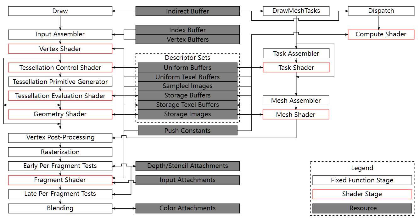
What does this pipeline look like in terms of processing stages? There are four main stage groups involved.

1. The CPU runs the application and the graphics driver. It is responsible for graphics pre-flight, such as animation and physics, uploading any CPU-generated data in to DRAM, and sending the rendering commands to the GPU.

2. The Command Processing stage is a control stage inside the GPU, responsible for interpreting the requests made by the CPU and coordinating the GPU’s data processing stages.

3. The Geometry Processing stage takes the input meshes designed by the content artists, animates each vertex into the correct location in screen-space, generates any additional per-vertex data payload such as per-vertex lighting, and emits a stream of primitives, most commonly triangles, for pixel processing to consume.

4. The Pixel Processing stage consumes this primitive data, rasterizes it to generate pixel coverage and executes the fragment coloring operations.

Geometry Processing

Vertex Shader

• Vertex Shading
• Projection

Tessellation Shaders

1. 控制着色器（Tessellation Control Shader, TCS）：
   • 它的主要任务是决定每个几何图形（如三角形、四边形等）应该被细分成多少更小的部分。
   • 控制着色器会输出细分因子，告诉后续的 tessellator 应该生成多少新的顶点或面。
2. 细分器（Tessellator）：
   • 这是一个固定的硬件单元，而不是可编程的着色器阶段。
   • 它根据控制着色器提供的细分因子来生成新的小的几何体（通常是更多的小三角形或四边形），将原始几何体划分成更精细的形状。
3. 评估着色器（Tessellation Evaluation Shader, TES）：
   • 这个阶段会对生成的几何图形进行最终调整和变形。
   • 评估着色器会根据生成的新顶点对它们的位置进行“拉扯”或“推挤”，以便将它们摆放到合适的位置，形成最终的形状。这一步通常用来实现曲面细化或其他几何变形效果。

Clipping

After the projection transform, only the primitives inside the unit cube (which correspond to primitives inside the view frustum) are needed for continued processing. Therefore, the primitives outside the unit cube are discarded, and primitives fully inside are kept. Primitives intersecting with the unit cube are clipped against the unit cube, and thus new vertices are generated and old ones are discarded.

After pre-rasterization shader stages, the following fixed-function operations are applied to vertices of the resulting primitives:

• Primitive clipping, including application-defined half-spaces (Primitive Clipping).
• Shader output attribute clipping (Clipping Shader Outputs).
• Clip space W scaling (Controlling Viewport W Scaling).
• Perspective division on clip coordinates (Coordinate Transformations).
• Viewport mapping, including depth range scaling (Controlling the Viewport).
• Front face determination for polygon primitives (Basic Polygon Rasterization).

Pixel Processing

Rasterization

D3D11 Rasterizer / Pixel Shader Attribute Interpolation Modes

In the Triangle Setup stage, the differentials, edge equations, and other data for the triangle are computed. These data may be used for triangle traversal, as well as for interpolation of the various shading data produced by the geometry stage. Fixed- function hardware is used for this task. Finding which samples or pixels are inside a triangle is often called Triangle Traversal. Each triangle fragment’s properties are generated using data interpolated among the three triangle vertices. These properties include the fragment’s depth, as well as any shading data from the geometry stage. It is also here that perspective-correct interpolation over the triangles is performed. All pixels or samples that are inside a primitive are then sent to the pixel processing stage.

Early Z

Early z test, late z update

zs test → fs: discard test → update z buffer and render target

Normal

zs test → update z buffer → fs → update render target

Coordinate Spaces

 In a rendering pipeline, a vertex typically goes through the following six coordinate spaces, each playing a specific role:

1. Object Space (Model Coordinates): This is the local coordinate system of the object itself. Vertices are defined relative to the object’s origin before any transformations.

   • Conversion: Apply the Model matrix, which transforms from object space to world space.

2. World Space: Vertices are now positioned in the global 3D scene, relative to the world origin.

   • Conversion: Use the View matrix to transform from world space to camera space.

3. Camera Space (View Coordinates): The scene is transformed relative to the camera’s position and orientation, centering the camera at the origin.

   • Conversion: Multiply by the Projection matrix to convert to clip space.

4. Clip Space: Vertices are projected onto a 2D plane, preparing for perspective division and clipping.

   • Conversion: After projection, the vertices undergo perspective division (divide by w) to move to NDC space.

5. Normalized Device Coordinates (NDC): Vertices are now in a normalized range of [-1, 1] for x, y, and z. This range corresponds to the visible area of the screen.

   • Conversion: Multiply NDC by the Viewport matrix to map to screen space.

6. Screen Space: NDC coordinates are transformed to pixel coordinates relative to the screen resolution, allowing rasterization to occur.

Clip coordinates for a vertex result from shader execution, which yields a vertex coordinate Position. Perspective division on clip coordinates yields normalized device coordinates,

Deferred Rendering

Forward Rendering

for obj
	for light
		for fragment
			CalculateLightColor(obj, light)
			
o*l*f

Forward + (Tile-based Forward) Rendering

• Depth prepass (prevent overdraw / provide tile depth bounds)
• Tiled light culling (output: light list per tile)
• Shading per object (PS: Iterate through light list calculated in light culling)

Deferred Rendering

for fragment
	for light
		CalculateLightColor(gbuffer, light)
l*f

A G-buffer (Geometry Buffer) is a set of textures that store various attributes of a scene's geometry during a deferred rendering pass. These attributes are used later for lighting calculations, allowing for more complex lighting models in deferred shading. The typical information stored in a G-buffer includes:

1. Position: Stores the 3D position of the geometry in either world space or view space. This allows reconstruction of the surface point during lighting calculations.

2. Normals: Stores the surface normal at each pixel. These normals are essential for calculating lighting effects like diffuse and specular reflections.

3. Albedo (Diffuse Color): Stores the base color of the material without lighting. This color is later combined with lighting information to produce the final pixel color.

4. Specular (or Glossiness): Stores information about the specular reflection properties of the surface, including the specular intensity and glossiness (shininess). This is used for calculating highlights.

5. Material Properties: Sometimes additional material properties like roughness, metallicity, or ambient occlusion are stored to enable more detailed shading models.

6. Depth (Z-buffer): Stores the depth (distance from the camera) for each pixel. This is often stored separately but can be included in the G-buffer for post-processing effects like depth of field or SSAO (Screen Space Ambient Occlusion).

In some implementations, other auxiliary information like emissive color or subsurface scattering properties may also be stored depending on the specific needs of the rendering engine.

Differences

• Forward Rendering: In forward rendering, shading calculations are performed before depth testing. When rendering n objects under m light sources, the computational complexity is O(n*m), meaning the number of lights significantly affects performance. Typically, in forward rendering, the fragment shader runs multiple times for each pixel.
• Deferred Rendering: In contrast, deferred rendering first performs depth testing, followed by shading calculations. Each pixel only runs the fragment shader once, resulting in better performance when dealing with multiple lights.

Pros

• Decouples Object and Light Complexity: Deferred rendering separates the complexity of light sources and objects. When rendering n objects with m light sources, the complexity is O(n + m), which is a significant reduction compared to forward rendering. Deferred rendering only calculates shading for visible pixels, which reduces the computational load.

• Efficient Use of Light Calculations: Instead of iterating through triangles and calculating lighting for each, deferred rendering first identifies all visible pixels and then applies lighting. This avoids unnecessary calculations for triangles that aren't visible, which is especially beneficial for scenes with many small or distant objects that don’t contribute to the final image.

• Avoids Inefficient Light Calculations: When rendering each pixel, you need to calculate whether the light reaches the pixel and what color is produced. In most cases, especially with point and spotlights, many of these calculations are unnecessary because the light doesn't affect the majority of pixels. By reducing these redundant calculations, deferred rendering improves efficiency.

Cons

• Not Suitable for Transparent Objects: Deferred rendering doesn't handle transparency well. The G-buffer stores the currently visible pixels, but for transparent objects, a single pixel may require storing more data, such as multiple depth values. Thus, deferred rendering usually handles opaque meshes first, with transparent objects rendered separately.

• High Memory Bandwidth Usage: Deferred rendering requires significant memory bandwidth. For example, with a resolution of 1920x1080, RGBA color format, 4 MRTs (Multiple Render Targets), and 60 FPS, the G-buffer can consume up to 15 GB of bandwidth. While this is manageable on desktop systems, it becomes a challenge on mobile devices.

• Uniform Lighting Pass: In deferred rendering, once the G-buffer is created, it's no longer possible to determine which pixel belongs to which mesh. This means all pixels must use the same lighting algorithm. In forward rendering, different meshes can use different lighting techniques, but deferred rendering lacks this flexibility. However, in most cases, a unified lighting approach is desired, so this limitation is often not a significant issue.

• Not friendly to MSAA

This organization highlights the key aspects of both rendering techniques, with deferred rendering offering more efficient lighting calculations but coming with challenges in transparency and memory usage.

Floating-Point Precision

"Floating-point" means that the decimal point can float, or move. Taking single-precision numbers as an example, ($1\times 10^{32}$) can only be accurate to the nearest whole number, while ($1\times 10^0$) can be accurate to 32 decimal places. This means that as numerical values increase, precision decreases.

During the rendering process, this lack of precision can cause errors in depth testing, where objects further from the camera may incorrectly appear in front of closer objects. This leads to rendering artifacts such as flickering or "broken" faces.

The simple solution to this is to move the model closer to the origin, which resolves the precision issue.

Z-Fighting

Z-fighting occurs when two surfaces are very close together in 3D space, and due to limited depth buffer precision, the renderer can't accurately determine which surface is in front of the other. This results in flickering or overlapping patterns as the renderer switches between the two surfaces.

• Reason: Depth values are typically stored as 24-bit or 32-bit floating-point numbers, but the precision is not distributed uniformly across the depth range. Precision is much higher closer to the camera (near clipping plane) and drops off as objects move farther away (toward the far clipping plane). When two surfaces are very close together at larger distances, the precision becomes insufficient to consistently distinguish which one is in front.

Reverse Z-buffering

• Reverse Z-buffering improves depth precision, especially for objects that are far from the camera.

• How it works: Normally, depth values are stored with more precision near the near plane and less precision near the far plane. Reverse Z flips this by using the far plane for higher precision, which reduces the chances of Z-fighting at a distance.

• Implementation:

  • Set the near clipping plane (zNear) to a small positive value and the far plane (zFar) to a large value.
  • Use a floating-point depth buffer (often 32-bit for better precision).
  • Reverse the depth calculation, so the depth values close to 1.0 are near the camera and those close to 0.0 are far away.
  • This is often combined with a GL_GREATER depth test (instead of GL_LESS), since higher precision is needed for distant objects.

  In OpenGL/Vulkan, this is achieved by setting the near-far range to [0, 1], using a reversed depth projection matrix, and ensuring the depth buffer uses floating-point precision.

SSAA and MSAA

A Quick Overview of MSAA

Rasterization Rules - Win32 apps | Microsoft Learn

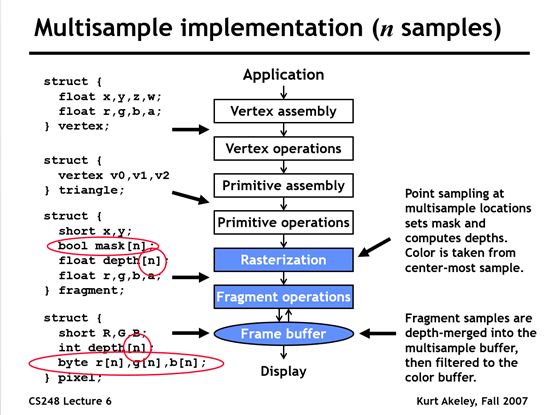
SSAA (Super-Sample Anti-Aliasing) can be understood as rendering at a higher resolution and then downsampling the image. The key difference between SSAA and MSAA is that SSAA shades every sample point, while MSAA shades each triangle per pixel only once.

During the rasterization phase, multiple sample points are used to determine whether a triangle covers the pixel. A coverage rate is then calculated. In the fragment shading stage, the color value is only calculated once for each pixel, based on the center of the pixel, but the final result is multiplied by the coverage rate. The efficiency of MSAA comes from not shading every sample point, but shading each pixel only once, and then applying the coverage rate to the final result.

However, MSAA doesn't work well with modern deferred shading frameworks. This is because, in deferred shading, the scene is rasterized into the G-buffer first, and shading is not directly performed. To force MSAA with deferred shading, you can check this SDK Sample.

Deferred Shading and MSAA

MSAA doesn't support deferred rendering very well.

MSAA operates during the rasterization phase, which occurs after the geometry stage but before the shading stage. It relies on the scene's geometric information. However, deferred rendering stores all scene information in the G-buffer first to optimize lighting calculations, so by the time shading occurs, the geometric information has already been discarded.

In the DirectX 9 era, MRT (Multiple Render Targets) didn't support MSAA. This support was added later with DirectX 10.1, allowing MSAA to be used with MRT.

Texture Sampling

LearnOpenGL - Textures

Filtering is the process of accessing a particular sample from a texture. There are two cases for filtering: minification and magnification.

Magnification means that the area of the fragment in texture space is smaller than a texel, and minification means that the area of the fragment in texture space is larger than a texel.

在 OpenGL 中，GL_TEXTURE_MIN_FILTER 和 GL_TEXTURE_MAG_FILTER 是用于控制纹理缩小和放大的插值方式的参数。

GL_TEXTURE_MIN_FILTER（纹理缩小过滤）

当纹理的像素比片元的像素多（即纹理被缩小时），需要进行纹理采样和插值。GL_TEXTURE_MIN_FILTER 选项有以下几种：

• GL_NEAREST：最近邻插值，选择最接近的纹素（Texel），不会进行插值，导致像素化效果。
• GL_LINEAR：线性插值，根据最近的 4 个纹素进行加权平均计算，使纹理更平滑。
• GL_NEAREST_MIPMAP_NEAREST：使用最接近的 Mipmap 级别，然后使用最近邻插值。
• GL_LINEAR_MIPMAP_NEAREST：使用最接近的 Mipmap 级别，然后进行线性插值。
• GL_NEAREST_MIPMAP_LINEAR：在两个最接近的 Mipmap 级别之间进行插值，然后用最近邻采样。
• GL_LINEAR_MIPMAP_LINEAR（三线性过滤）：在两个最接近的 Mipmap 级别之间进行插值，然后用线性插值获取最终颜色，效果最平滑。

GL_TEXTURE_MAG_FILTER（纹理放大过滤）

当纹理的像素比片元的像素少（即纹理被放大时），需要插值计算新像素。可用的选项有：

• GL_NEAREST：最近邻插值，选择最接近的纹素，不进行平滑处理，可能会产生马赛克效果。
• GL_LINEAR：线性插值，根据周围的 4 个纹素加权平均，使纹理更平滑。

注意：

• GL_TEXTURE_MAG_FILTER 只能 选择 GL_NEAREST 或 GL_LINEAR，不支持 Mipmap 相关的选项。
• Mipmap 仅在缩小时生效，因此 GL_TEXTURE_MIN_FILTER 允许使用 Mipmap 选项，而 GL_TEXTURE_MAG_FILTER 不支持。

如果你的程序使用 Mipmap 但 GL_TEXTURE_MIN_FILTER 仅设置为 GL_NEAREST 或 GL_LINEAR，你需要调用 glGenerateMipmap(GL_TEXTURE_2D); 以确保 Mipmap 级别自动生成。

The magnification filter is controlled by the GL_TEXTURE_MAG_FILTER texture parameter. This value can be GL_LINEAR or GL_NEAREST. If GL_NEAREST is used, then the implementation will select the texel nearest the texture coordinate; this is commonly called "point sampling". If GL_LINEAR is used, the implementation will perform a weighted linear blend between the nearest adjacent samples.

The minification filter is controlled by the GL_TEXTURE_MIN_FILTER texture parameter. When doing minification, you can choose to use mipmapping or not.

The baseline texture filter that is really used in content is a bilinear filter, the GL_LINEAR_MIP_NEAREST filter in OpenGL ES.

Each sample reads 4 texels from a single mipmap level, in a 2x2 pattern, and blends them based on distance to the sample point. This is fastest filter supported by a Mali GPU, giving full speed throughput and the lowest texture bandwidth.

The next level of filter used is a trilinear filter, or the GL_LINEAR_MIP_LINEAR filter in OpenGL ES.

Each sample makes two bilinear samples from the two nearest mipmap levels, and then blends those together. This runs at half the speed of a basic bilinear filter, and may require up to 5 times the bandwidth for some samples as they will fetch data from a more detailed mipmap.

Bilinear (GL_LINEAR_MIP_NEAREST)

Anisotropic 2x bilinear (GL_LINEAR_MIP_NEAREST)

Trilinear (GL_LINEAR_MIP_LINEAR)

Anisotropic 2x trilinear (GL_LINEAR_MIP_LINEAR)

Anisotropic 3x bilinear (GL_LINEAR_MIP_NEAREST)

Anisotropic 3x trilinear (GL_LINEAR_MIP_LINEAR)

Anisotropic Filtering: Improves image clarity by considering the non-square (anisotropic) nature of the pixel filter footprint.

LOD Calculation Texture Filter Anisotropic

Ripmaps and summed area tables

• Can look up axis-aligned rectangular zones
• Diagonal footprints are still a problem

EWA filtering

• Use multiple lookups
• Weighted average
• Mipmap hierarchy still helps
• Can handle irregular footprint

Fragments and Pixels

• Pixel: A pixel is a specific point on the screen and is the smallest displayable unit on a device. It is ultimately colored and displayed to the user.
• Fragment: A fragment is generated during the rasterization stage and represents part of a triangle that covers a certain pixel's area. Each fragment contains attributes related to the triangle (such as color, depth, and texture coordinates), but it has not yet determined the final color of that pixel.

When a triangle is rasterized, multiple fragments might be generated to cover the same pixel. If multi-sample anti-aliasing (MSAA) is enabled, each pixel has multiple samples, and each fragment might partially or fully cover those samples. SV_Coverage calculates which samples of the pixel are covered by the current fragment.

In simple terms, a fragment is an intermediate state related to geometry and pixel coverage, while a pixel is the final output shown on the screen. In multi-sampling, one pixel can be covered by multiple fragments, and different fragments may affect different samples within the same pixel.

• Fragment（片段）

  • 光栅化的产物：在顶点处理、图元装配后，图形管线通过光栅化（Rasterization）将几何图元（如三角形）分解为离散的片段。
  • 候选像素：每个片段对应屏幕空间中的一个潜在像素位置，但尚未通过最终测试（如深度测试、模板测试、透明度混合等）。
  • 携带元数据：片段包含颜色、深度、纹理坐标等信息，供片段着色器（Fragment Shader）处理。

• Pixel（像素）

  • 最终的显示单元：像素是帧缓冲区（Framebuffer）中的实际存储单元，代表屏幕上最终显示的颜色值。
  • 通过测试的片段：只有通过所有测试（如深度测试）且未被丢弃的片段，才会成为像素写入帧缓冲区。

关键区别

特性	Fragment（片段）	Pixel（像素）
阶段	光栅化后，测试前（中间状态）	测试与混合后（最终状态）
存在形式	临时数据，可能被修改或丢弃	帧缓冲区中的稳定值
数量关系	一个像素可能对应多个片段（如抗锯齿）	一个像素对应屏幕上一个显示点
操作位置	片段着色器（Fragment Shader）	帧缓冲区（直接操作需特殊技术）

• 片段的作用：每个像素包含多个子样本（片段），最终通过加权平均生成平滑的像素颜色。
• 结果：一个像素可能由多个片段组合而成，但最终显示为一个像素值。

简而言之，片段是像素的候选者，而像素是片段的胜利者。

Radiometry

• Radiant Energy $Q$
  • Energy of electromagnetic radiation. (Rarely used in CG)
  • Units: Joule (J)
• Radiant Flux (Power) $\Phi =\frac{\mathrm{d}Q}{\mathrm{d}t}$
  • Energy per unit time.
  • Units: Watt (W), lumen (lm)
• Radiant Intensity $I(\omega )=\frac{\mathrm{d}\Phi }{\mathrm{d}\omega }$
  • Power per unit solid angle.
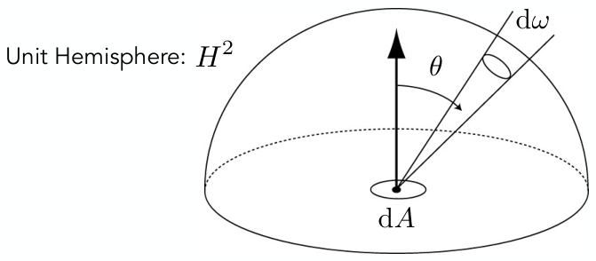
• Solid Angle $\Omega =\frac{A}{r^2}$
  • Ratio of subtended area on a sphere to radius squared.
• Differential Solid Angles
  • $d\omega =\frac{dA}{r^2}=\sin \theta d\theta d\varphi$
    • $\mathrm{d}A=(r\mathrm{d}\theta )(r\sin \theta \mathrm{d}\varphi )=r^2\sin \theta \mathrm{d}\theta \mathrm{d}\varphi$
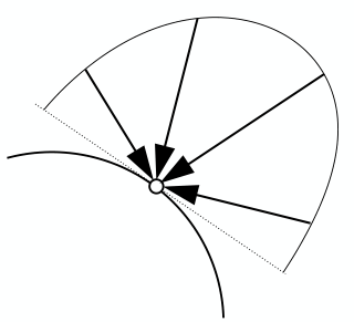
    • Sphere: $\Omega ={\int }_0^{2\pi }{\int }_0^{\pi }\sin \theta \mathrm{d}\theta \mathrm{d}\varphi =4\pi$
    • When $\theta$ and $\varphi$ change by a small amount, the resulting differential solid angle is not simply $\mathrm{d}\theta \mathrm{d}\varphi$; it depends on $\sin \theta$. This means the change in solid angle varies depending on whether the direction in spherical coordinates is closer to the "pole" or the "equator," reflecting the uneven division of surface area by $\theta$ and $\varphi$.
• Irradiance $E(\mathbf{x})=\frac{\mathrm{d}\Phi (\mathbf{x})}{\mathrm{d}A}$
  • Power per projected unit area.
  • Units: $\frac{\mathrm{W}}{{\mathrm{m}}^2}$ (lux: $\frac{\text{lm}}{{\mathrm{m}}^2}$)
• Radiance (Luminance) $L(\mathrm{p},\omega )=\frac{{\mathrm{d}}^2\Phi (\mathrm{p},\omega )}{\mathrm{d}\omega \mathrm{dA}\cos \theta }$
  • Power per unit solid angle, per projected unit area.
  • Units: $\frac{\mathrm{W}}{\mathrm{sr}\cdot {\mathrm{m}}^2}$ (nit: $\frac{\mathrm{cd}}{{\mathrm{m}}^2}=\frac{\mathrm{lm}}{\mathrm{sr}\cdot {\mathrm{m}}^2}$)

Irradiance Falloff

When power from a point light source is uniformly distributed over a spherical shell, the irradiance at any point decreases according to $r^2$. This means that it's actually the irradiance that falls off with distance. A common misconception is that intensity falls off, which is incorrect; intensity is the power per unit solid angle and does not decrease with distance.

Incident Radiance / Exiting Radiance

Incident radiance is the irradiance per unit solid angle arriving at the surface. $L(\mathrm{p},\omega )=\frac{\mathrm{d}E(\mathrm{p})}{\mathrm{d}\omega \cos \theta }$ i.e. it is the light arriving at the surface along a given ray (point on surface and incident direction).

Exiting surface radiance is the intensity per unit projected area leaving the surface.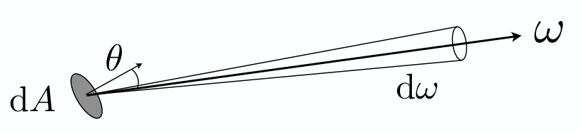 $L(\mathrm{p},\omega )=\frac{\mathrm{d}I(\mathrm{p},\omega )}{\mathrm{d}A\cos \theta }$ e.g. for an area light it is the light emitted along a given ray (point on surface and exit direction).

Irradiance vs. Radiance

Irradiance: total power received by area $\mathrm{d}A$

Radiance: power received by area $\mathrm{d}A$ from "direction" $\mathrm{d}\omega$

$$\begin{array}{rl}dE(\mathrm{p},\omega )& =L_i(\mathrm{p},\omega )\cos \theta \mathrm{d}\omega \\ E(\mathrm{p})& ={\int }_{H^2}{L}_i(\mathrm{p},\omega )\cos \theta \mathrm{d}\omega \end{array}$$

• Intensity: Power per solid angle.
• Irradiance: Power per projected unit area.
• Radiance:
  • Irradiance per unit solid angle.
  • Intensity per projected unit area.

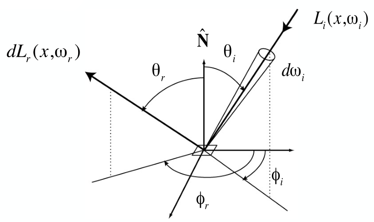
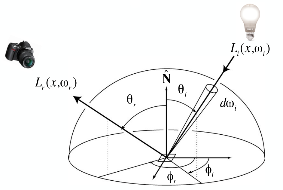
Bidirectional Reflectance Distribution Function (BRDF)

$\frac{\mathrm{d}{L}_r({\omega }_r)}{\mathrm{d}{E}_i({\omega }_i)}$ is the Bidirectional Reflectance Distribution Function (BRDF), a measure of how much light a surface reflects from a specific incoming direction ${\omega }_i$ to a specific outgoing direction ${\omega }_r$. Physically, it describes the ratio of radiance $L_r$ (the power per unit area per unit solid angle) in the outgoing direction to irradiance $E_i$ (the power per unit area) from the incoming direction.

$$f_r({\omega }_i\to {\omega }_r)=\frac{\mathrm{d}{L}_r({\omega }_r)}{\mathrm{d}{E}_i({\omega }_i)}=\frac{\mathrm{d}{L}_r({\omega }_r)}{L_i({\omega }_i)\cos {\theta }_i\mathrm{d}{\omega }_i}$$

Units: $\frac{1}{\mathrm{sr}}$

BRDF描述的是材质的一种固有光学属性，它需要将出射的“亮度”与真正“到达并被表面接收”的能量关联起来，而到达表面的能量密度是由辐照度（Irradiance）来衡量的，而非入射的辐射亮度（Radiance）本身。

Diffuse / Lambertian Material

$$\begin{array}{rl}& L_o({\omega }_o)={\int }_{H^2}{f}_r{L}_i({\omega }_i)\cos {\theta }_i\mathrm{d}{\omega }_i\\ & =f_r{L}_i{\int }_{H^2}\cos {\theta }_i\mathrm{d}{\omega }_i\\ & =\pi f_r{L}_i\end{array}$$ $$f_r=\frac{\rho }{\pi }$$

$\rho$ represents the surface's reflectance or albedo, which is the proportion of light that an object reflects.

Note: The integral ${\int }_{H^2}\cos {\theta }_i\mathrm{d}{\omega }_i=\pi$. To ensure energy conservation, the diffuse BRDF must divide by $\pi$. Otherwise, the output radiance $L_o$ would be $\pi$ times the input radiance $L_i$.

The Rendering Equation

The Reflection Equation

$$L_r(\mathrm{p},{\omega }_r)={\int }_{H^2}{f}_r(\mathrm{p},{\omega }_i\to {\omega }_r)L_i(\mathrm{p},{\omega }_i)\cos {\theta }_i\mathrm{d}{\omega }_i$$

The Rendering Equation

$$L_o(x,{\omega }_o)=L_e(x,{\omega }_o)+{\int }_{\Omega }{L}_i(x,{\omega }_i)f(x,{\omega }_i,{\omega }_o)\cos {\theta }_i\mathrm{d}{\omega }_i$$

The meaning of each term in the equation is as follows:

1. $L_r(x,{\omega }_r)$: Reflected Light (Output Image)
   • The reflected light, or the light intensity seen from point $x$ in the direction ${\omega }_r$. This is usually the color of the image we observe.
2. $L_e(x,{\omega }_r)$: Emission
   • Emission, the light emitted from point $x$ in the direction ${\omega }_r$. This term represents self-emitting objects, like light sources or materials with self-emission.
3. ${\int }_{\Omega }$: Integral over Hemisphere $\Omega$
   • Integration over the incident light direction ${\omega }_i$ in the hemisphere $\Omega$, considering light arriving at point $x$ from all directions.
4. $L_i(x,{\omega }_i)$: Incident Light (from light source)
   • Incident light, the light intensity arriving at point $x$ from direction ${\omega }_i$.
5. $f(x,{\omega }_i,{\omega }_r)$: BRDF (Bidirectional Reflectance Distribution Function)
   • The Bidirectional Reflectance Distribution Function (BRDF), which describes how light incident from direction ${\omega }_i$ at point $x$ is reflected in direction ${\omega }_r$.
6. $\cos {\theta }_i$: Cosine of Incident Angle
   • The cosine of the incident angle ${\theta }_i$, representing the angle between the incident direction ${\omega }_i$ and the surface normal. This term accounts for the effect of the light's angle on its intensity.
7. $d{\omega }_i$: Differential Solid Angle
   • A small differential solid angle element used to integrate over the direction ${\omega }_i$ on the hemisphere.

This equation describes the light intensity observed at point $x$ from direction ${\omega }_r$ as a combination of self-emission and the accumulation of reflected incident light from all directions.

Rendering Equation as Integral Equation

• The rendering equation is expressed as: $L_o(x,{\omega }_o)=L_e(x,{\omega }_o)+{\int }_{\Omega }{L}_i(x,{\omega }_i)f(x,{\omega }_i,{\omega }_o)\cos \theta d{\omega }_i$
• Where:
  • $L_o$: Reflected light (output image) – unknown.
  • $L_e$: Emission – unknown.
  • $L_i$: Reflected light – unknown.
  • $f$: Bidirectional Reflectance Distribution Function (BRDF) – known.
  • $\cos \theta$: Cosine of incident angle – known.
• This equation is a Fredholm integral equation of the second kind, which can be expressed in canonical form and solved numerically.

Linear Operator Equation

• The equation form is: $I(u)=e(u)+\int I(v)K(u,v)dv$ where $K(u,v)$ is the kernel (light transport operator).
• The rendering equation can be represented as: $L=E+KL$This can be discretized into a simple matrix equation or system of simultaneous linear equations, where $L$ and $E$ are vectors, and $K$ is the light transport matrix.

Ray Tracing and Extensions

• Ray tracing is a general class of numerical Monte Carlo methods.
• It approximates all possible light paths in the scene:
  • $L=E+KL$
  • $(I-K)L=E$
  • $L=(I-K{)}^{-1}E$
• Using the Binomial Theorem, further expansion gives: $L=(I+K+K^2+K^3+\dots )E=E+KE+K^{2}E+K^{3}E+\dots$* Each term represents different types of illumination:
  • $E$: Direct emission from light sources.
  • $KE$: Direct illumination on surfaces.
  • $K^{2}E$: Single-bounce indirect illumination (reflections/refractions).
  • $K^{3}E$: Two-bounce indirect illumination.

Shading in Rasterization

• In rasterization, only direct emission from light sources and direct illumination on surfaces are considered.

PBR

PBR Theory

漫反射部分为什么要除以一个 π？

是因为：

$${\int }_{2\pi }\cos {\theta }_{o}d{\omega }_o=\pi$$

如果散射的光线最后都能汇集到一点的话，积分的结果就是会再乘一个 pi。所以分散的时候就需要除 pi。

对半球积分

$${\int }_0^{2\pi }{\int }_0^{\frac{\pi }{2}}\sin (\theta )\cos (\theta )d\theta d\varphi =\pi$$

$2\pi {\int }_0^{\frac{\pi }{2}}\cos (x)\sin (x)dx$, $u=\sin (x)$ , $=\int udu=\frac{u^2}{2}=2\pi {\int }_0^{\frac{\pi }{2}}\frac{si{n}^{2}x}{2}=\frac{1}{2}\times 2\pi =\pi$

Blinn-Phong

Blinn-Phong 高光使用dot(norm, halfwayDir)。具有更平滑的高光效果，并且更稳定，不容易出现镜面闪烁的问题。

Phong 用dot(viewDir, reflectDir)。当光源和视点位于同一个方向时，反射光线跟观察方向可能大于 90 度，反射光线的分量就被消除了，在处理高光时会出现光照不连续的情况。

https://learnopengl.com/img/advanced-lighting/advanced_lighting_comparrison.png

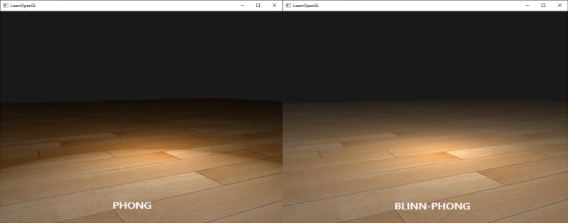
// ambient
vec3 ambient = lightColor * material.ambient;
 
// diffuse
vec3 norm = normalize(Normal);
vec3 lightDir = normalize(lightPos - FragPos);
float diff = max(dot(norm, lightDir), 0.0);
vec3 diffuse = lightColor * (diff * material.diffuse);
 
// specular
vec3 viewDir = normalize(viewPos - FragPos);
vec3 reflectDir = reflect(-lightDir, norm);
 
if (PHONG) {
  float spec = pow(max(dot(viewDir, reflectDir), 0.0), material.shininess);
} else if (BLINN_PHONG) {
  vec3 halfwayDir = normalize(lightDir + viewDir);
  float spec = pow(max(dot(norm, halfwayDir), 0.0), material.shininess);
}
 
vec3 specular = lightColor * (spec * material.specular);
 
vec3 result = ambient + diffuse + specular;

公式如下：

$$\begin{gathered} L=L_a+L_d+L_s \\ =k_a{I}_a+k_d\left(\frac{I}{r^2}\right)\max (0,\mathbf{n}\cdot \mathbf{l})+k_s\left(\frac{I}{r^2}\right)\max (0,\mathbf{n}\cdot \mathbf{h}{)}^p \end{gathered}$$

其中：

• $L$：最终光照强度
• $L_a$（环境光）、$L_d$（漫反射光）、$L_s$（镜面反射光）分别表示不同光照贡献
• $k_a,k_d,k_s$：环境光、漫反射和镜面反射系数
• $I_a$：环境光强度
• $I$：光源强度
• $r$：光源到表面的距离
• $\mathbf{n}$：表面法向量
• $\mathbf{l}$：指向光源的方向向量
• $\mathbf{h}$：半程向量（观察方向和光照方向的中间向量）
• $p$：高光指数（决定高光的锐利程度）

Rasterization vs Ray Tracing

注重质量，面光源，软阴影

Rasterization is not the only computer rendering technique today. A well-known alternative is ray tracing, often used for high-quality rendering in cases where rendering time is less critical. While efforts have been made to commercialize real-time ray tracing GPUs, they have so far been relatively unsuccessful and remain an area of academic research.

Strengths of Rasterization

• Simplicity: The primary strength of rasterization is its simplicity.
• Scalability: Rasterization scales to more complex scenes by adding hardware.
• Hardware Acceleration: In hardware-accelerated rasterization, the majority of processing happens independently:
  • Vertices: Processed independently of other vertices.
  • Framebuffer fragments: Coloring operations are only dependent on fragments at the same screen location (requiring depth, stencil, and color info for correct writeback).
• Amdahl’s Law: Graphics APIs are designed with minimal serialization points, allowing for efficient parallelization. This enables rasterization to handle more vertices and pixel operations as more GPU cores are added.
• Highly Parallelizable: Graphics rendering is one of the few algorithms that can scale well by adding more cores. The only limits are silicon area, power budget, and the memory system's ability to supply data to the GPU.

Weaknesses of Rasterization

• Limited Basis in Real-World Physics: Rasterization, beyond handling 3D coordinate data, has little connection to actual physics.
  • Accurate Rendering: High-quality rendering requires understanding how light interacts with objects to determine surface light intensity and color, which involves factors like shadows, reflections, and refractions.
• Global Knowledge: Rasterization lacks the global knowledge needed to automatically handle effects like shadows. It cannot determine whether one triangle is in the shadow of another while rendering because it focuses only on the triangle at hand.
• Mimicking Reality: Many advanced rendering effects (e.g., lighting, shadows, reflections) are mimics of reality in rasterization. These effects:
  • Require developers to insert extra geometry or rendering passes.
  • Are designed to look realistic, even if the method of achieving them differs from real-world physics.
• Performance Trade-Off: While these emulations can look convincing, they are generally faster than achieving the same results with ray tracing, which "does it properly."

Conclusion:

Rasterization is fast and scalable, making it the dominant choice for real-time rendering. However, ray tracing is a more physically accurate alternative, suitable for scenarios where visual quality is prioritized over performance.

Shadow Map

Cause of Shadow Acne

自适应Shadow Bias算法 - 知乎

A 2-Pass Algorithm

• Pass 1: Render from Light， Output a “depth texture” from the light source

• Pass 2: Render from Eye

  • Render a standard image from the eye
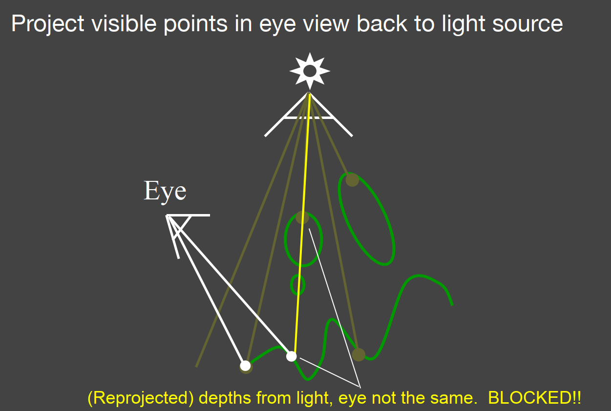
  • Project visible points in eye view back to light source
  • (Reprojected) depths match for light and eye. VISIBLE
  • (Reprojected) depths from light, eye not the same. BLOCKED

Pro: no knowledge of scene’s geometry is required

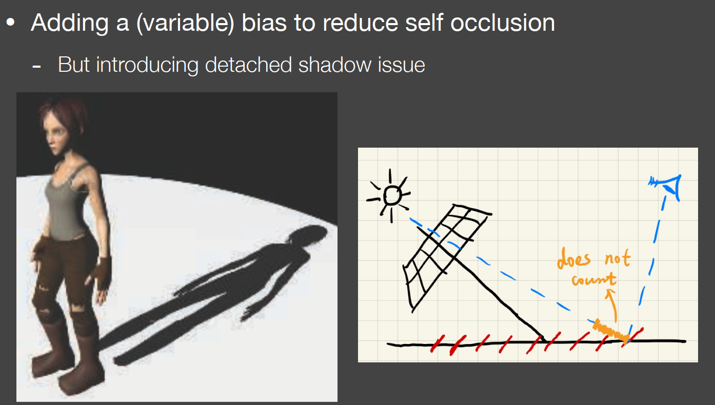
Con: causing self occlusion and aliasing issues

由于深度图具有固定的分辨率，因此深度通常每个纹素跨越多个片段。结果，多个片段从深度图中采样相同的深度值并得出相同的阴影结论，从而产生这些锯齿状的块状边缘。

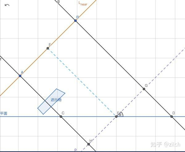
我们暂且假设 Light 对应的正交矩阵其宽高相同,记为 frustumSize。ShadowMap 贴图的尺寸记为 shadowMapSize。

影响最大 Bias 的两个因素如下:

• ShadowMap 的分辨率
• 平行光的入射角

设图中 AB 线段代表 ShadowMap 贴图上单位像素在 Light 近平面上对应的尺寸。那么我们有以下公式:

|AB| = frustumSize / shadowMapSize

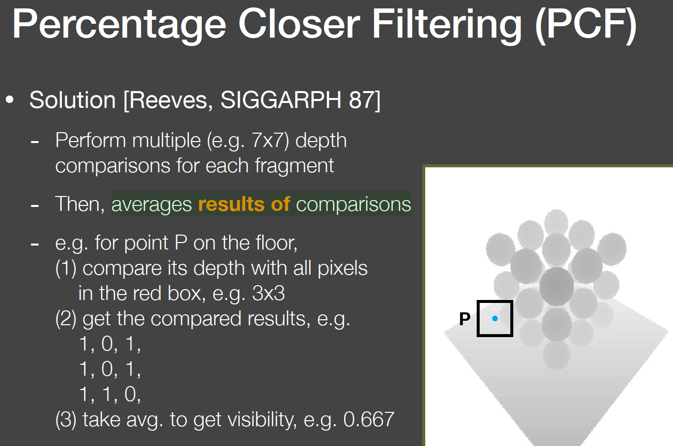
Percentage Closer Filtering

Provides anti-aliasing at shadows’ edges

Filtering the results of shadow comparisons

平均深度比较结果

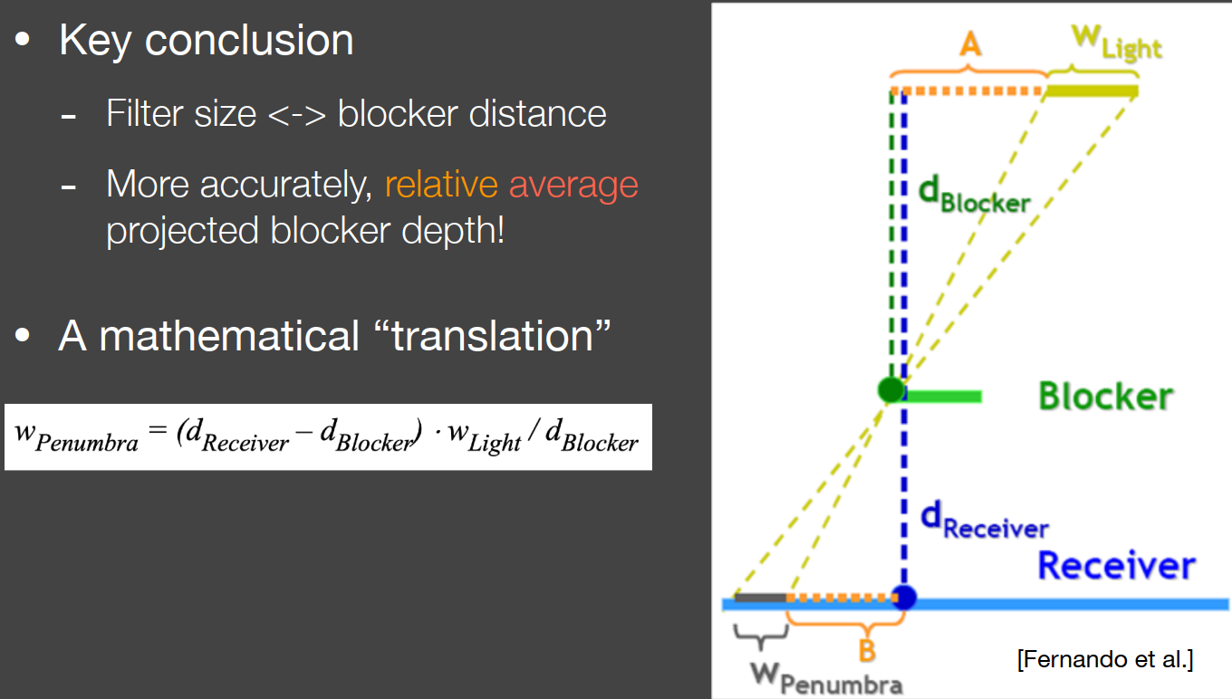
Percentage Closer Soft Shadows

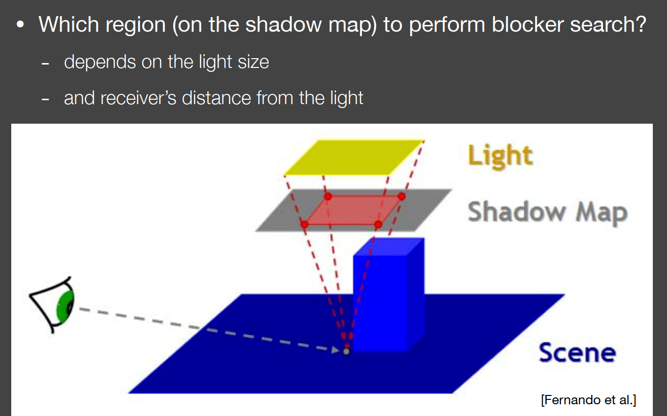
Which region (on the shadow map) to perform blocker search?

Shadowmap 的常见问题：

a. 阴影抖动问题，可以通过偏移技术来解决，增加一个 bias 来比较片段深度，还有更好的一种方式是使用一种自适应偏移的方案，基于斜率去计算当前深度要加的偏移；

b. 阴影锯齿问题，可以使用百分比渐进过滤(Percentage Closer Filter，PCF)技术进行解决：从深度贴图中多次采样，每次采样坐标都稍有些不同，比如上下左右各取 9 个点进行采样（即一个九宫格），最后加权平均处理，就可以得到柔和的阴影。标准 PCF 算法采样点的位置比较规则，最后呈现的阴影还是会看出一块一块的 Pattern（图块），可以采用一些随机的样本位置，比如 Poisson Disk 来改善 PCF 的效果

c. 采样 Shadowmap 的时候，需要将标准设备坐标系的坐标范围由[-1,1]修正到[0,1]，否则贴图的坐标范围是[0,1]，会采样错误。

百分比渐进软阴影 (Percentage-Closer Soft Shadows, PCSS)

通过控制 PCF 的 Kernel Size，就可以改变阴影的模糊半径，进而模拟出软阴影的效果，这就是 PCSS 算法的思路。之所以有软阴影，是因为某些区域处于光源的半影区（Penumbra），所以 PCSS 算法会设法估算出当前位置的半影区大小，这个大小决定了 PCF 算法的 Kernel Size，最终呈现出一个视觉上的软阴影效果。

空间加速

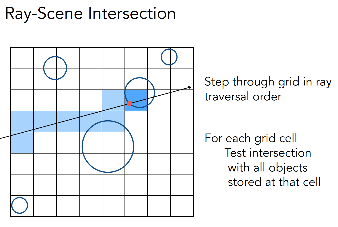
Uniform Grids

在 AABB 里面划分小格子，然后预处理将物体包含的格子做标记；接着遍历光线上的格子，在计算光线与标记过的格子中的物体是否相交。这样可以省略对那些不包含格子的物体进行求交计算，进一步提高求交速度：

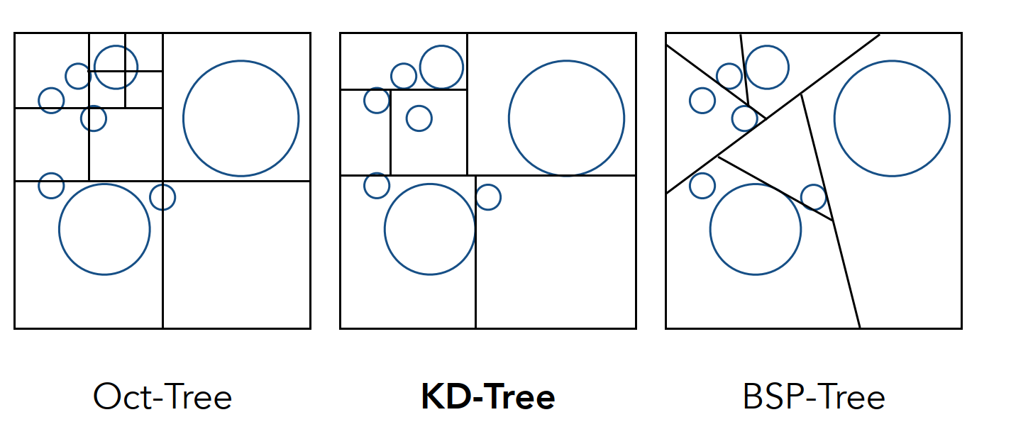
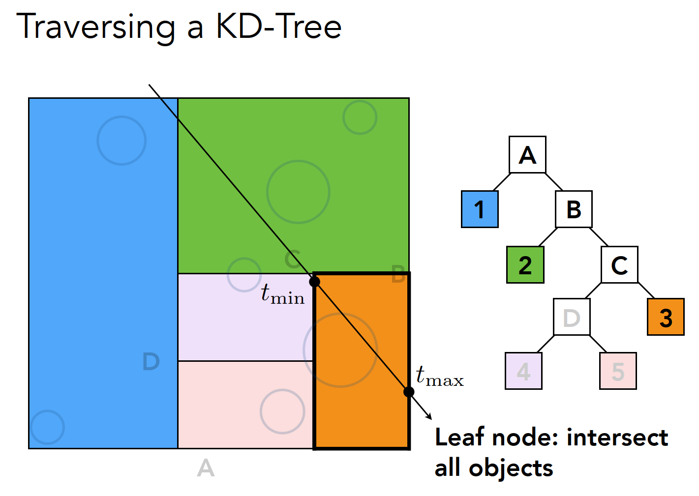
八叉树、KD 树

空间进行划分，将对象组织称为二叉树/四叉树/八叉树/KD 树的数据结构：

Bounding Volume Hierarchy

基于对象进行划分，目前得到最广泛的应用：

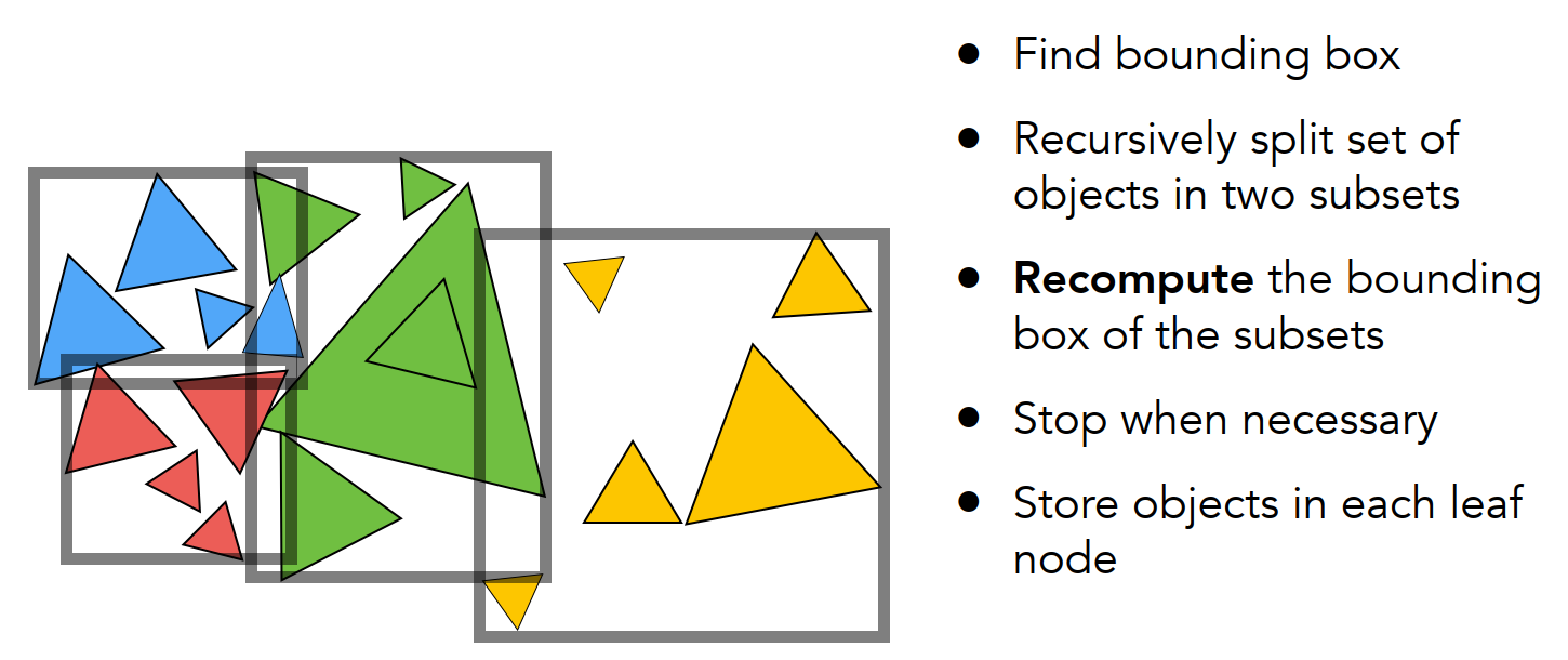
How to subdivide a node?

• Choose a dimension to split(类似于 KD-Tree，沿着某个维度划分)
• Heuristic #1：Always choose the longest axis in node(使最后的划分结果比较均匀)
• Heuristic #2: Split node at location of median object (用某种方式将这堆三角形排好，取第 n/2 个三角形，使得两边三角形个数尽可能差不多，树尽可能平衡，树的最大深度尽可能小，这样平均搜索的次数就少了；这便涉及到一个排序问题，如何将这堆三角形排序？快速选择算法-O(n))

Termination criteria/什么时候划分结束?

• Heuristic: stop when node contains few elements(e.g., 5)

使用 BVH 可以避免一个对象同时存在不同的包围盒/区域中，以下是根据空间划分和根据对象进行划分的算法区别：

Spatial partition（e.g., KD-Tree）

• Partition space into non-overlapping regions
• An object can be contained in multiple regions

Object partitions(e.g., BVH)

• Partition set of objects into disjoint subsets
• Bounding boxes for each set may overlap in space

后处理

1. 景深（Depth of Field）：景深是指相机对焦点前后相对清晰的成像范围。在计算机图形学中，景深效果可以通过模拟光学相机的焦距和光圈来实现，使得渲染的图像中的部分物体或景观模糊，从而使得焦点以外的物体看起来更加真实。景深效果通常用于模拟摄影效果，增强图像的艺术感和真实感。
2. 运动模糊（Motion Blur）：运动模糊效果模拟快速运动物体在图像上留下的模糊轨迹。这种效果可以增加动态感和真实感，特别是在动画和游戏中。运动模糊效果可以通过模拟相机快门速度或物体运动轨迹来实现。
3. 光晕（Bloom）：光晕效果模拟了亮度较高的区域周围的光晕效果。它可以使得图像中的光源或亮部分看起来更加柔和和明亮，增加图像的动态范围和视觉吸引力。光晕效果通常通过将图像中的亮部分进行高斯模糊并叠加到原始图像上来实现。
4. 色调映射（Tone Mapping）：色调映射效果用于调整图像的色调和对比度，以使得图像在不同的显示设备上呈现出更好的视觉效果。它通常用于处理高动态范围（HDR）图像，将其转换为低动态范围（LDR）图像，以便更好地显示在标准的显示器上。

伽马校正

Understanding Gamma Correction

Gamma变换

• 显示器的输出在 Gamma2.2 空间。
• sRGB 对应 Gamma0.45 空间。
• 伽马校正和显示器输出平衡之后，结果就是 Gamma1.0 的线性空间。

Math

Projection Matrix

OpenGL Projection Matrix

投影矩阵 P(Projection)：将顶点坐标从观察空间变换到裁剪空间(clip space) [-w,w] 后续的透视除法操作会将裁剪空间的坐标转换为标准化设备坐标系中（NDC） [-1,1]

平截头体经过透视投影变换后再进行正交变换时，内部点的 $z$ 值会更偏向于远平面还是近平面呢？

对于点 $(x,y,z,1)$，透视投影矩阵 $M_{\text{persp}\to \text{ortho}}$ 的第三行计算得到：

$$z^{\prime }=(n+f)z-nf$$

而第四行计算得到：

$$w^{\prime }=z$$

因此，透视除法后新的 $z$ 值为：

$$f(z)=\frac{z^{\prime }}{w^{\prime }}=\frac{(n+f)z-nf}{z}=n+f-\frac{nf}{z}$$

我们进行边界条件验证：

• 当 $z=n$ 时：

  $$f(n)=n+f-\frac{nf}{n}=n$$

• 当 $z=f$ 时：

  $$f(f)=n+f-\frac{nf}{f}=f$$

这表明近平面和远平面上的点，其 $z$ 值未发生变化。

现在我们分析 $f(z)$ 在区间 $0<n<z<f$ 内的大小关系。
由于 $n,f$ 均为正数，我们考察不等式：

$$n+f-\frac{nf}{z}>z$$

整理得：

$$n+f>z+\frac{nf}{z}$$

即：

$$z^2-(n+f)z+nf<0$$

所以根的表达式为：

$$z=\frac{(n+f)\pm |n-f|}{2}$$

根据 $n<f$，我们得到两个根：

$$z_1=\frac{(n+f)-(f-n)}{2}=n,z_2=\frac{(n+f)+(f-n)}{2}=f$$

该二次函数开口向上，在 $z\in (n,f)$ 的范围内恒成立，因此：

$$f(z)>z,\forall z\in (n,f)$$

这说明经过变换后，视锥体内部的点在 $z$ 方向上被压缩得更偏向远平面 $f$。

View Transformation

相机坐标变换矩阵

Lecture 04 Transformation Cont

OpenGL Camera

We assume that $\vec{g}\perp \vec{l}$, meaning the gaze direction is perpendicular to the up direction. In practice, the camera's up direction is defined manually. Our goal is to align the look-at direction with the negative z-axis and the up direction with the positive y-axis.

This process is called view transformation (or camera transformation), and it is represented as $M_{\text{view}}$, where:

$$M_{\text{view}}=R_{\text{view}}{T}_{\text{view}}$$

First, we perform a translation (where $\vec{e}=(x_e,y_e,z_e)$ represents the position of the camera in the scene):

$$T_{\text{view}}=\left(\begin{array}{cccc}1& 0& 0& -x_e\\ 0& 1& 0& -y_e\\ 0& 0& 1& -z_e\\ 0& 0& 0& 1\end{array}\right)$$

Next, we perform a rotation. We rotate the gaze direction $\vec{g}$, the up direction $\hat{t}$, and their cross product $\hat{g}\times \hat{t}$ to align with the Z, Y, and X axes, respectively. The inverse rotation $R_{\text{view}}^{-1}$ can be written as:

$$R_{\text{view}}^{-1}=\left(\begin{array}{cccc}{x}_{\hat{g}\times \hat{t}}& x_{\hat{t}}& x_{\widehat{-g}}& 0\\ y_{\hat{g}\times \hat{t}}& y_{\hat{t}}& y_{\widehat{-g}}& 0\\ z_{\hat{g}\times \hat{t}}& z_{\hat{t}}& z_{\widehat{-g}}& 0\\ 0& 0& 0& 1\end{array}\right)$$

Since rotation matrices are orthogonal, we know that:

$$R_{\text{view}}=(R_{\text{view}}^{-1}{)}^T=\left(\begin{array}{cccc}{x}_{\hat{g}\times \hat{t}}& y_{\hat{g}\times \hat{t}}& z_{\hat{g}\times \hat{t}}& 0\\ x_{\hat{t}}& y_{\hat{t}}& z_{\hat{t}}& 0\\ x_{\widehat{-g}}& y_{\widehat{-g}}& z_{\widehat{-g}}& 0\\ 0& 0& 0& 1\end{array}\right)$$

Finally, by substituting the rotation and translation matrices, we get the complete view transformation matrix $M_{\text{view}}$.

Projection Transformation

Once the camera and objects are positioned correctly, the next step is to project the 3D objects onto a 2D plane. There are two main types of projection: orthographic projection and perspective projection. The projection transformations discussed below map a cuboid to the space of $[-1,1{]}^3$.

Orthographic Projection

Orthographic projection can be understood as:

• The camera is positioned at the origin, looking along the negative Z-axis, with the up direction aligned with the Y-axis.
• The Z-axis of the object is discarded.
• The object is scaled and translated to fit within the $[-1,1{]}^2$ range (meaning the x and y axes are confined between -1 and 1).

Consider the cuboid defined by $[l,r]\times [b,t]\times [f,n]$. The goal is to scale and translate it into the canonical cube $[-1,1{]}^3$. The orthographic projection matrix is:

$$M_{\text{ortho}}=\left[\begin{array}{cccc}\frac{2}{r-l}& 0& 0& 0\\ 0& \frac{2}{t-b}& 0& 0\\ 0& 0& \frac{2}{n-f}& 0\\ 0& 0& 0& 1\end{array}\right]\left[\begin{array}{cccc}1& 0& 0& -\frac{r+l}{2}\\ 0& 1& 0& -\frac{t+b}{2}\\ 0& 0& 1& -\frac{n+f}{2}\\ 0& 0& 0& 1\end{array}\right]$$

Perspective Projection

The perspective projection follows these steps:

1. $M_{\text{persp}\to \text{ortho}}$: The frustum is "squeezed" into a cube, ensuring that points on the near plane remain unchanged, and the z-coordinate of points on the far plane remains the same. The z-coordinates of points between the near and far planes will change.
2. $M_{\text{ortho}}$: Apply the orthographic projection described above.

The final projection matrix is $M_{\text{persp}}=M_{\text{ortho}}{M}_{\text{persp}\to \text{ortho}}$.

Deriving $M_{\text{persp}\to \text{ortho}}$

Let $(x,y,z)$ be a point in the frustum. After applying $M_{\text{persp}\to \text{ortho}}$, this point is transformed to $\left(\frac{nx}{z},\frac{ny}{z},\text{unknown}\right)$, meaning:

$$M_{\text{persp}\to \text{ortho}}\left(\begin{array}{c}x\\ y\\ z\\ 1\end{array}\right)=\left(\begin{array}{c}\frac{nx}{z}\\ \frac{ny}{z}\\ \text{unknown}\\ 1\end{array}\right)=\left(\begin{array}{c}nx\\ ny\\ \text{unknown}\\ z\end{array}\right)$$

Thus, $M_{\text{persp}\to \text{ortho}}$ has the form:

$$M_{\text{persp}\to \text{ortho}}=\left(\begin{array}{cccc}n& 0& 0& 0\\ 0& n& 0& 0\\ ?& ?& ?& ?\\ 0& 0& 1& 0\end{array}\right)$$

Given that points on the near plane remain unchanged and the z-coordinate on the far plane remains constant, we have:

$$M_{\text{persp}\to \text{ortho}}\left(\begin{array}{c}x\\ y\\ n\\ 1\end{array}\right)=\left(\begin{array}{c}x\\ y\\ n\\ 1\end{array}\right)=\left(\begin{array}{c}nx\\ ny\\ n^2\\ n\end{array}\right)$$ $$M_{\text{persp}\to \text{ortho}}\left(\begin{array}{c}0\\ 0\\ f\\ 1\end{array}\right)=\left(\begin{array}{c}0\\ 0\\ f\\ 1\end{array}\right)=\left(\begin{array}{c}0\\ 0\\ f^2\\ f\end{array}\right)$$

Solving these, we get:

$$M_{\text{persp}\to \text{ortho}}=\left(\begin{array}{cccc}n& 0& 0& 0\\ 0& n& 0& 0\\ 0& 0& n+f& -nf\\ 0& 0& 1& 0\end{array}\right)$$

Computing $l$, $r$, $b$, $t$ from fovY and Aspect Ratio

Instead of defining the near plane using $l$ (left), $r$ (right), $b$ (bottom), and $t$ (top) coordinates, we can use the field-of-view (fovY) and aspect ratio. The following relations hold:

$$\begin{array}{rl}& t=|n|\tan \left(\frac{\text{fovY}}{2}\right)\\ & r=t\cdot \text{aspect}\\ & b=-t,l=-r\end{array}$$

This defines the near plane in terms of field-of-view and aspect ratio.

Normal Transformation Matrix

The Normal Matrix

In realistic lighting calculations, model vertex normals are typically used. Lighting can be computed in either the view space or world space. A key advantage of performing lighting calculations in the view space is that the observer's (i.e., the camera's) position is always at $(0,0,0)$.

Let's assume lighting is calculated in view space. The transformation from local space to view space is represented by $MV$ (where $M$ is the model matrix, and $V$ is the view matrix).

In a vertex shader, input data includes vertex positions (localPosition) and normals (N), both of which are in the local space. The vertex position in the view space is computed as:

$$MV\cdot localPosition$$

However, for the vertex normal in view space, simply applying $MV\cdot N$ is incorrect. For example, if the model undergoes non-uniform scaling, applying $MV\cdot N$ would result in a vector that is no longer perpendicular to the surface—thus no longer a valid normal.

The Correct Normal Transformation Matrix

The matrix used to transform normals from local space to view space is the transpose of the inverse of the vertex transformation matrix $MV$, denoted as:

$$G={\left((MV{)}^{-1}\right)}^T$$

If lighting calculations are done in world space, the normal matrix becomes ${\left(M^{-1}\right)}^T$.

Normals Transformed by Modelview Matrix

(proof of $(M^{-1}{)}^T$ transform)

Point $(x,y,z,w)$ is on a plane in 3D (homogeneous coordinates) if and only if

$$ax+by+cz+dw=0,$$

or

$$[abcd]\left[\begin{array}{c}x\\ y\\ z\\ w\end{array}\right]=0.$$

Now, let's transform the plane by $M$.

Point $(x,y,z,w)$ is on the transformed plane if and only if

$$M^{-1}\left[\begin{array}{c}x\\ y\\ z\\ w\end{array}\right]$$

is on the original plane:

$$[abcd]M^{-1}\left[\begin{array}{c}x\\ y\\ z\\ w\end{array}\right]=0.$$

So, the equation of the transformed plane is:

$$[a^{\prime }{b}^{\prime }{c}^{\prime }{d}^{\prime }]\left[\begin{array}{c}x\\ y\\ z\\ w\end{array}\right]=0,$$

for

$$\left[\begin{array}{c}{a}^{\prime }\\ b^{\prime }\\ c^{\prime }\\ d^{\prime }\end{array}\right]=(M^{-1}{)}^T\left[\begin{array}{c}a\\ b\\ c\\ d\end{array}\right].$$

Special Cases and Performance Considerations

In some cases, such as when the model undergoes only rotation and translation (no scaling), the transformation matrix $MV$ can be used directly for normal transformation. This is because the upper-left $3\times 3$ matrix of $MV$ is an orthogonal matrix, meaning:

$$(MV{)}^{-1}=(MV{)}^T\Rightarrow G=MV$$

Optimization

Computing the inverse matrix is computationally expensive and unsuitable for calculating the normal matrix for every vertex or pixel in vertex or fragment shaders. Instead, the inverse-transpose matrix can be precomputed once on the CPU and passed as a uniform variable to the shader.

Additionally, this article points out that in most common cases, we don't need to explicitly compute the normal matrix. We can use the adjugate matrix's transpose as the normal matrix.

The adjugate matrix always exists. The inverse of a matrix is the adjugate matrix divided by the matrix's determinant. If the determinant is zero (i.e., the matrix is singular), the inverse doesn't exist, but the adjugate matrix still does.

Therefore, the adjugate matrix's transpose can be used as the normal transformation matrix. The difference between the adjugate and inverse matrices is just a scaling factor, which only affects the length of the transformed normal vector. The adjugate matrix always exists, so we can safely use it as the normal matrix, but we should normalize the transformed normal afterward to ensure unit length.

2D Rotation

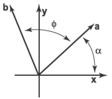
Suppose we want to rotate a vector a by an angle $\varphi$ counterclockwise to get vector b. If a makes an angle $\alpha$ with the $x$-axis, and its length is $r=\sqrt{x_a^2+y_a^2}$ , then we know that

$$\begin{gathered} x_a=r\cos \alpha , \\ {y}_a=r\sin \alpha . \end{gathered}$$

Because b is a rotation of a, it also has length $r$. Because it is rotated an angle $\varphi$ from a, b makes an angle $(\alpha +\varphi )$ with the $x$-axis. Using the trigonometric addition identities:

$$\begin{gathered} x_b=r\cos (\alpha +\varphi )=r\cos \alpha \cos \varphi -r\sin \alpha \sin \varphi , \\ {y}_b=r\sin (\alpha +\varphi )=r\sin \alpha \cos \varphi +r\cos \alpha \sin \varphi . \end{gathered}$$

Substituting $x_a=r\cos \alpha$ and $y_a=r\sin \alpha$ gives

$$\begin{gathered} x_b=x_a\cos \varphi -y_a\sin \varphi , \\ {y}_b=y_a\cos \varphi +x_a\sin \varphi . \end{gathered}$$

In matrix form, the transformation that takes a to b is then

$$\text{rotate}(\varphi )=\left[\begin{array}{cc}\cos \varphi & -\sin \varphi \\ \sin \varphi & \cos \varphi \end{array}\right].$$

Reflection Vector Calculation

Vector Calculation Method

Let:

• $\vec{I}$ be the incident ray vector
• $\vec{N}$ be the normal vector (a unit vector perpendicular to the surface)
• $\vec{R}$ be the reflected ray vector

The formula for the reflected ray is:

$$\vec{R}-\vec{I}=-2(\vec{I}\cdot \vec{N})\vec{N}$$

This can be understood as follows:

• $(\vec{I}\cdot \vec{N})$ is the dot product, which gives the projection of $\vec{I}$ onto $\vec{N}$
• $-2(\vec{I}\cdot \vec{N})\vec{N}$ represents twice this projection in the direction of $\vec{N}$
• Subtracting $\vec{I}$ from $\vec{R}$ gives the twice-reflected component

Thus, the reflected ray vector is:

$$\vec{R}=\vec{I}-2(\vec{I}\cdot \vec{N})\vec{N}$$

Angle Method

This method focuses on the angles of incidence and reflection.

Let:

• $\theta$ be the angle between the incident ray and the normal
• $\varphi$ be the azimuthal angle (the angle in the plane of the surface)

Key points:

• The angle of incidence equals the angle of reflection: ${\theta }_{incident}={\theta }_{reflected}$
• The azimuthal angle of the reflected ray is opposite to that of the incident ray: ${\varphi }_{reflected}={\varphi }_{incident}+180^{\circ }$

This method is particularly useful when:

• Working in spherical coordinates
• The surface normal is aligned with one of the coordinate axes

Point Within a Triangle (Polygon)

$$\text{叉乘}(V_1,V_2)=(x_1,y_1)\times (x_2,y_2)=x_1{y}_2-y_1{x}_2$$ $$\vec{a}\times \vec{b}=A^{\ast }b=\left(\begin{array}{ccc}0& -z_a& y_a\\ z_a& 0& -x_a\\ -y_a& x_a& 0\end{array}\right)\left(\begin{array}{c}{x}_b\\ y_b\\ z_b\end{array}\right)$$

Barycentric 坐标

给定一个三角形 $△ABC$，其中三个顶点的坐标分别为：

$$A(x_A,y_A),B(x_B,y_B),C(x_C,y_C)$$

那么，任意平面上的点 $P(x,y)$ 可以用 Barycentric 坐标 $({\lambda }_1,{\lambda }_2,{\lambda }_3)$ 来表示：

$$P={\lambda }_{1}A+{\lambda }_{2}B+{\lambda }_{3}C$$

其中 ${\lambda }_1,{\lambda }_2,{\lambda }_3$ 满足：

$${\lambda }_1+{\lambda }_2+{\lambda }_3=1$$

这表示 $P$ 是顶点的线性组合。

Barycentric 坐标可以通过面积法或者向量叉积来计算。最常见的方法是利用三角形面积：

$${\lambda }_1=\frac{\text{Area}(△PBC)}{\text{Area}(△ABC)}$$ $${\lambda }_2=\frac{\text{Area}(△PAC)}{\text{Area}(△ABC)}$$ $${\lambda }_3=\frac{\text{Area}(△PAB)}{\text{Area}(△ABC)}$$

由于三角形面积可以用向量叉积表示：

$$\text{Area}(△XYZ)=\frac{1}{2}|(X-Z)\times (Y-Z)|$$

其中向量叉积 $(X-Z)\times (Y-Z)$ 计算的是 2D 叉积：

$$(X-Z)\times (Y-Z)=(x_X-x_Z)(y_Y-y_Z)-(y_X-y_Z)(x_Y-x_Z)$$

所以可以得到：

$${\lambda }_1=\frac{(x_B-x_C)(y-y_C)-(y_B-y_C)(x-x_C)}{(x_B-x_C)(y_A-y_C)-(y_B-y_C)(x_A-x_C)}$$ $${\lambda }_2=\frac{(x_C-x_A)(y-y_C)-(y_C-y_A)(x-x_C)}{(x_B-x_C)(y_A-y_C)-(y_B-y_C)(x_A-x_C)}$$ $${\lambda }_3=1-{\lambda }_1-{\lambda }_2$$

如何判断点在三角形内

根据 Barycentric 坐标的性质，点 $P$ 在三角形内部当且仅当：

$$0\le {\lambda }_1\le 1,0\le {\lambda }_2\le 1,0\le {\lambda }_3\le$$

如果任何一个 $\lambda$ 超出范围，说明点 $P$ 在三角形外部。

• 如果所有 $\lambda$ 在 [0,1] 之间，则 $P$ 在三角形内部或边界上。
• 如果有一个 $\lambda$ 小于 0 或大于 1，则 $P$ 在三角形外部。

直观理解

Barycentric 坐标的本质是用顶点的加权平均来表示一个点的位置：

• ${\lambda }_1$ 代表 $A$ 对点 $P$ 位置的影响
• ${\lambda }_2$ 代表 $B$ 对点 $P$ 位置的影响
• ${\lambda }_3$ 代表 $C$ 对点 $P$ 位置的影响

如果 $P$ 在三角形内，每个点都贡献一部分权重，并且权重之和为 1；如果 $P$ 在三角形外，就会出现负的权重，表明它更接近三角形外的区域。

Negative Bary-check

可以通过向量 叉积（cross product） 来判断：

1. 计算 三角形三个顶点到点 P 的向量
2. 计算 每条边与该向量的叉积
3. 如果 所有叉积的方向一致（点积结果全为正或全为负），说明 P 在三角形内，否则在外

这种方法利用 叉积方向不变性，避免了浮点误差带来的问题。

• Negative Bary-check 是一种 更稳健的三角形内部点检测方法，通过检查重心坐标的 负值 或 叉积方向 来判断。

Ray Intersection With Plane

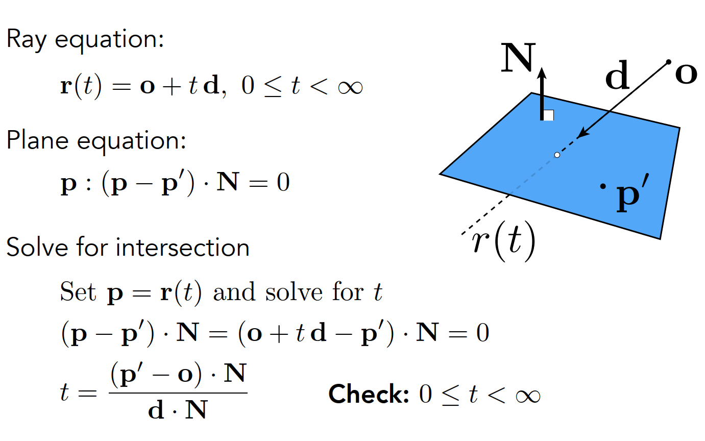
Ray Intersection With Triangle

Triangle is in a plane

• Ray-plane intersection
• Test if hit point is inside triangle

Möller Trumbore Algorithm

如果一个点在三角形内，就能用重心坐标系去表示这个点；带入方程，有 3 个未知数（b1，b2，t），得到三个等式；解出这三个未知数；判定 t 是否合理，t > 0，然后(1-b1-b2), b1, b2 are barycentric coordinates，就是有解。

$$\vec{\mathbf{O}}+t\vec{\mathbf{D}}=(1-b_1-b_2){\vec{\mathbf{P}}}_0+b_1{\vec{\mathbf{P}}}_1+b_2{\vec{\mathbf{P}}}_2$$ $$\left[\begin{array}{c}t\\ b_1\\ b_2\end{array}\right]=\frac{1}{{\vec{\mathbf{S}}}_1\bullet {\vec{\mathbf{E}}}_1}\left[\begin{array}{c}{\vec{\mathbf{S}}}_2\bullet {\vec{\mathbf{E}}}_2\\ {\vec{\mathbf{S}}}_1\bullet \vec{\mathbf{S}}\\ {\vec{\mathbf{S}}}_2\bullet \vec{\mathbf{D}}\end{array}\right]$$ $$\begin{array}{rl}& {\vec{\mathbf{E}}}_1={\vec{\mathbf{P}}}_1-{\vec{\mathbf{P}}}_0\\ & {\vec{\mathbf{E}}}_2={\vec{\mathbf{P}}}_2-{\vec{\mathbf{P}}}_0\\ & \vec{\mathbf{S}}=\vec{\mathbf{O}}-{\vec{\mathbf{P}}}_0\\ & {\vec{\mathbf{S}}}_1=\vec{\mathbf{D}}\times {\vec{\mathbf{E}}}_2\\ & {\vec{\mathbf{S}}}_2=\vec{\mathbf{S}}\times {\vec{\mathbf{E}}}_1\end{array}$$

Cost = (1 div, 27 mul, 17 add)

Recall: How to determine if the intersection isinside the triangle?

Hint: (1-b1-b2), b1, b2 are barycentric coordinates!

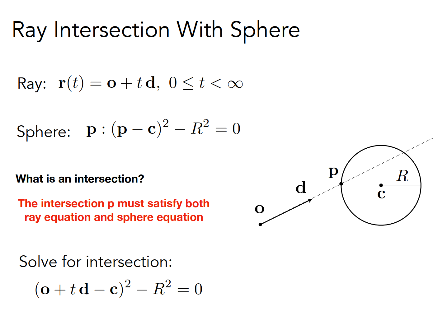
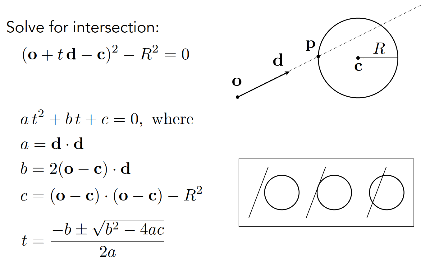
Ray Intersection With Sphere

Ray Intersection with Axis-Aligned Box (AABB)

• A 3D box can be represented as three pairs of infinitely large slabs.
• Ray enters the box only when it enters all pairs of slabs.
• Ray exits the box as soon as it exits any pair of slabs. Intersection Calculation

1. For each slab pair, compute tmin and tmax (negative values are allowed).
2. For the 3D box:
   • tenter = max{tmin} (largest entry point)
   • texit = min{tmax} (smallest exit point)
   • If tenter < texit, the ray stays inside the box for a while, meaning there is an intersection.

• A ray is not a mathematical line, so we must check physical correctness of t values. - If texit < 0:
  - The box is behind the ray → No intersection. - If texit >= 0 and tenter < 0:
  - The ray originates inside the box → Intersection occurs. Conclusion A ray intersects an AABB if and only if: tenter < texit && texit >= 0

两个三角形相交

1. 分别检查每个三角形的边与另一个三角形的边是否相交：

   • 对于每个三角形，检查它的三条边是否与另一个三角形的三条边相交。如果存在相交的边，则两个三角形相交。
   • 如果两个三角形相交，必定至少其中一个三角形的一条边穿过了另一个三角形的内部；把边当作光线去跟另一个三角形求交，如果三条边只要有一条边跟三角形有交点，即可判断两三角形相交，当然关键是要判断计算出来的 t 是否合理，是否位于边长范围之内。

2. 使用分离轴定理：

   • 分离轴定理指出，如果两个凸多边形（如三角形）在某一轴上都是分离的，那么它们不相交。可以检查两个三角形在所有可能的轴上是否分离，如果没有找到分离轴，则它们相交。

齐次坐标

所谓齐次坐标就是为矢量或者矩阵增加一个维度，2D 平面使用 3 维向量和三维矩阵，3D 空间使用 4 维向量和 4 维矩阵；额外的坐标值是任意的，可以看作缩放或者权重。

三维矩阵可以表示旋转和缩放，它们相乘的结果是正确的，但是平移变换不能加到三维矩阵中的相乘去表达，只能将矩阵相乘的结果加一个三维向量；引入齐次坐标之后会增加一个维度，变为四维矩阵，多出来的一维向量用来表示平移，那么就可以在一个矩阵中统一所有的操作：平移、旋转、缩放。

Unified way to represent all transformations.

欧拉角、矩阵、四元数表示旋转的区别

1. 欧拉角：
   • 表示方式：欧拉角使用三个角度来描述旋转，通常包括绕三个坐标轴的旋转角度（例如，绕 x y z 轴的旋转角度）。
   • 优点：直观易懂，可以直接对应于人类感知的旋转概念，易于理解和可视化。单个维度上的角度比较容易插值
   • 缺点：存在万向锁问题（Gimbal Lock），某些组合旋转可能会导致失去自由度。另外，在数学上，欧拉角存在歧义，因为不同的旋转顺序会导致不同的结果。
2. 旋转矩阵：
   • 表示方式：旋转矩阵是一个 3x3 的正交矩阵，描述了旋转变换对应的线性变换。
   • 优点：不受万向锁问题的影响，没有歧义，而且可以直接与向量相乘以实现旋转变换。内置的硬件加速点积和矩阵乘法
   • 缺点：不太直观，需要更多的存储空间，也不太容易进行插值计算，而且矩阵运算相对耗费计算资源。
3. 四元数：
   • 表示方式：四元数是一种复数扩展，由一个实部和三个虚部构成，通常记为 q = (w, x, y, z)。在旋转表示中，单位四元数描述了绕某个轴的旋转。
   • 优点：没有万向锁问题，避免了欧拉角的歧义，而且在进行旋转插值时效率较高。四元数的好处是能够串接旋转；能把旋转直接作用于点或者矢量；而且能够进行旋转插值；另外它所占用的存储空间也比矩阵小；四元数可以解决万向节死锁的问题。
   • 缺点：相对于欧拉角来说，直观性稍差一些。同时，四元数的计算和理解相对复杂一些。

切线空间

顶点法线切线UV和三角面 | Xhhfp

切线空间（Tangent Space） 是一个局部坐标空间，用于表示模型表面上某点附近的方向。它的核心目的是将 法线、切线、和副切线（Binormal/Bitangent） 组成一个正交基，以便在着色或光照计算时进行更方便的向量变换。

顶点着色器：计算 TBN

// 顶点着色器中传递 TBN
out vec3 vTangent;
out vec3 vBitangent;
out vec3 vNormal;
 
// 计算 TBN
vec3 dp1 = dFdx(position);
vec3 dp2 = dFdy(position);
vec2 duv1 = dFdx(texCoords);
vec2 duv2 = dFdy(texCoords);
 
vec3 tangent = normalize(duv2.y * dp1 - duv1.y * dp2);
vec3 bitangent = normalize(duv1.x * dp2 - duv2.x * dp1);
vec3 normal = normalize(cross(tangent, bitangent));
 
// 传递给片段着色器
vTangent = tangent;
vBitangent = bitangent;
vNormal = normal;

片段着色器：法线变换

// 从法线贴图中读取法线
vec3 normalMap = texture(normalMapSampler, texCoords).rgb * 2.0 - 1.0;
 
// 创建 TBN 矩阵
mat3 TBN = mat3(normalize(vTangent), normalize(vBitangent), normalize(vNormal));
 
// 转换法线到世界空间
vec3 worldNormal = normalize(TBN * normalMap);

切线空间（Tangent Space）通常用于法线贴图（Normal Mapping），以便在模型表面上正确地应用法线方向。切线空间的计算主要依赖于 顶点位置、UV 坐标 和 法线，其核心在于构造 切线（Tangent）、副切线（Bitangent，也叫 BiNormal） 和 法线（Normal） 三个向量，从而形成一个局部坐标系。下面是详细计算过程：

计算切线空间（Tangent Space）

假设给定一个三角形的三个顶点 ${\mathbf{p}}_0,{\mathbf{p}}_1,{\mathbf{p}}_2$ 及其对应的 UV 坐标 $(u_0,v_0),(u_1,v_1),(u_2,v_2)$，计算切线（Tangent）和副切线（Bitangent）的过程如下：

计算边向量

$${\mathbf{E}}_1={\mathbf{p}}_1-{\mathbf{p}}_0,{\mathbf{E}}_2={\mathbf{p}}_2-{\mathbf{p}}_0$$

计算 UV 坐标变化量

$$\Delta u_1=u_1-u_0,\Delta v_1=v_1-v_0$$ $$\Delta u_2=u_2-u_0,\Delta v_2=v_2-v_0$$

计算切线（Tangent） 和 副切线（Bitangent）

定义线性系统：

$${\mathbf{E}}_1=\mathbf{T}\Delta u_1+\mathbf{B}\Delta v_1$$ $${\mathbf{E}}_2=\mathbf{T}\Delta u_2+\mathbf{B}\Delta v_2$$

将其转换为矩阵求解：

$$\left[\begin{array}{c}\mathbf{T}\\ \mathbf{B}\end{array}\right]={\left[\begin{array}{cc}\Delta u_1& \Delta v_1\\ \Delta u_2& \Delta v_2\end{array}\right]}^{-1}\left[\begin{array}{c}{\mathbf{E}}_1\\ {\mathbf{E}}_2\end{array}\right]$$

求解：

$$\mathbf{T}=\frac{1}{\Delta u_1\Delta v_2-\Delta u_2\Delta v_1}(\Delta v_2{\mathbf{E}}_1-\Delta v_1{\mathbf{E}}_2)$$ $$\mathbf{B}=\frac{1}{\Delta u_1\Delta v_2-\Delta u_2\Delta v_1}(-\Delta u_2{\mathbf{E}}_1+\Delta u_1{\mathbf{E}}_2)$$

其中 $\mathbf{T}$ 是切线向量，$\mathbf{B}$ 是副切线向量。

归一化

$$\mathbf{T}=\frac{\mathbf{T}}{||\mathbf{T}||},\mathbf{B}=\frac{\mathbf{B}}{||\mathbf{B}||}$$

至此，我们得到了三角形的 切线（Tangent）和副切线（Bitangent）。

在你给出的公式中，我们首先通过线性系统来解出切线（$\mathbf{T}$）和副切线（$\mathbf{B}$）。但是，由于计算过程中并没有直接强制这两个向量正交，因此得到的结果不一定是正交的。为了确保它们是正交的，可以进行以下处理

正交化过程

1. 切线和副切线正交化： 在计算得出切线和副切线后，你可以使用正交化方法（例如Gram-Schmidt正交化）来强制它们变得正交。 具体地说，可以对$\mathbf{B}$向量执行如下操作：

   $${\mathbf{B}}_{\text{ortho}}=\mathbf{B}-(\mathbf{T}\cdot \mathbf{B})\mathbf{T}$$

   然后，归一化${\mathbf{B}}_{\text{ortho}}$，使其成为单位向量：

   $${\mathbf{B}}_{\text{ortho}}=\frac{{\mathbf{B}}_{\text{ortho}}}{||{\mathbf{B}}_{\text{ortho}}||}$$

   这样，$\mathbf{T}$和${\mathbf{B}}_{\text{ortho}}$将是正交的。

2. 确保切线和副切线的规范化： 切线和副切线都应该是单位向量，这就是你在后续步骤中的归一化操作，保证了它们的长度是1。

应用法线贴图

法线贴图存储的是切线空间中的法线，通常在纹理中以 RGB 形式存储：

• $R$（红色通道） → 切线方向分量 ($x$)
• $G$（绿色通道） → 副切线方向分量 ($y$)
• $B$（蓝色通道） → 法线方向分量 ($z$)

在着色器中，我们需要将 切线空间法线转换到世界空间，然后用于光照计算。转换过程如下：

通常法线贴图的 RGB 值存储在 $[0,1]$ 之间，因此需要转换到 $[-1,1]$：

${\mathbf{N}}_{\mathbf{T}}=2\times {\mathbf{N}}_{tex}-1$

这将法线贴图数据转换为切线空间中的法线方向。

用计算得到的 Tangent（T）、Bitangent（B） 和 法线（N） 构造一个变换矩阵：

$$\mathbf{TBN}=\left[\begin{array}{ccc}{T}_x& B_x& N_x\\ T_y& B_y& N_y\\ T_z& B_z& N_z\end{array}\right]$$

这个矩阵可以将切线空间的法线转换到 世界空间 或 视图空间。

$${\mathbf{N}}_{\mathbf{W}}=\mathbf{TBN}\cdot {\mathbf{N}}_{\mathbf{T}}$$

其中：

• ${\mathbf{N}}_{\mathbf{T}}$ 是法线贴图提供的切线空间法线
• ${\mathbf{N}}_{\mathbf{W}}$ 是转换到世界空间的法线，之后可以用于光照计算

总结

1. 计算切线空间（Tangent Space）：从顶点位置和 UV 计算切线（Tangent）、副切线（Bitangent）、法线（Normal）。
2. 使用法线贴图：
   • 采样法线贴图并转换到 $[-1,1]$ 空间。
   • 构造 TBN 矩阵，将法线从切线空间转换到世界空间。
   • 用世界空间法线进行光照计算。

点乘

点乘公式

1. 分量形式：
   对于向量 $\mathbf{a}=(a_1,a_2,\dots ,a_n)$ 和 $\mathbf{b}=(b_1,b_2,\dots ,b_n)$，点乘为：

   $$\mathbf{a}\cdot \mathbf{b}=a_1{b}_1+a_2{b}_2+\cdots +a_n{b}_n$$

2. 几何形式：
   用模长和夹角表示：

   $$\mathbf{a}\cdot \mathbf{b}=|\mathbf{a}||\mathbf{b}|\cos \theta$$

   其中 $\theta$ 是两向量间的夹角。点乘为0时，两向量垂直。

投影计算

向量 $\mathbf{a}$ 在 $\mathbf{b}$ 方向上的投影长度为：

$$\text{投影长度}=\frac{\mathbf{a}\cdot \mathbf{b}}{|\mathbf{b}|}$$

或等价于 $|\mathbf{a}|\cos \theta$。

向量 $\mathbf{a}$ 在 $\mathbf{b}$ 方向上的投影向量为：

$${\text{proj}}_{\mathbf{b}}\mathbf{a}=\left(\frac{\mathbf{a}\cdot \mathbf{b}}{\mathbf{b}\cdot \mathbf{b}}\right)\mathbf{b}$$

其中，$\mathbf{b}\cdot \mathbf{b}=|\mathbf{b}{|}^2$，分母为标量，分子为点乘结果。

• 投影公式
  • A · B / |A| 给出 B 在 A 方向上的标量投影（有符号长度）。
  • A · B / |B| 给出 A 在 B 方向上的标量投影。
  • 点积具有交换律 (A · B = B · A)，因此这两个投影概念是对称的。关键在于除以哪个向量的模长，就得到另一个向量在该向量方向上的投影长度。
• 投影分数/百分比 (Projection Fraction)
  • 计算$\frac{\mathbf{a}\cdot \mathbf{b}}{|\mathbf{b}{|}^2}$，也就是点积除以 B 模长的平方。
  • 意义： 这个结果表示“A 在 B 方向上的投影长度”占“B 自身总长度”的比例或分数（例如 0.45）。
  • 用途：
    1. 有时直接需要这个比例值。
    2. 优化： 计算模长平方比计算模长 (|B| = sqrt(...)) 快得多，因为它避免了开销较大的开平方根 (sqrt) 运算。在某些场景下，用比例代替实际投影长度是一种性能优化。

推导

我们可以从余弦定理的公式

$$c^2=a^2+b^2-2ab\cos \theta$$

推导出点乘的分量形式。

设有两个向量：

$$\mathbf{a}=(a_1,a_2,\dots ,a_n),\mathbf{b}=(b_1,b_2,\dots ,b_n)$$

向量的模长（欧几里得范数）定义为：

$$|\mathbf{a}|=\sqrt{a_1^2+a_2^2+\cdots +a_n^2},|\mathbf{b}|=\sqrt{b_1^2+b_2^2+\cdots +b_n^2}$$

两向量之差为：

$$\mathbf{c}=\mathbf{a}-\mathbf{b}=(a_1-b_1,a_2-b_2,\dots ,a_n-b_n)$$

其模长为：

$$|\mathbf{c}{|}^2=(a_1-b_1{)}^2+(a_2-b_2{)}^2+\cdots +(a_n-b_n{)}^2$$

根据余弦定理：

$$|\mathbf{c}{|}^2=|\mathbf{a}{|}^2+|\mathbf{b}{|}^2-2|\mathbf{a}||\mathbf{b}|\cos \theta$$

展开 $|\mathbf{c}{|}^2$：

$$|\mathbf{c}{|}^2=(a_1-b_1{)}^2+(a_2-b_2{)}^2+\cdots +(a_n-b_n{)}^2$$ $$=a_1^2-2a_1{b}_1+b_1^2+a_2^2-2a_2{b}_2+b_2^2+\cdots +a_n^2-2a_n{b}_n+b_n^2$$ $$=(a_1^2+a_2^2+\cdots +a_n^2)+(b_1^2+b_2^2+\cdots +b_n^2)-2(a_1{b}_1+a_2{b}_2+\cdots +a_n{b}_n)$$

由于：

$$|\mathbf{a}{|}^2=a_1^2+a_2^2+\cdots +a_n^2,|\mathbf{b}{|}^2=b_1^2+b_2^2+\cdots +b_n^2$$

所以：

$$|\mathbf{c}{|}^2=|\mathbf{a}{|}^2+|\mathbf{b}{|}^2-2(a_1{b}_1+a_2{b}_2+\cdots +a_n{b}_n)$$

与余弦定理比较：

$$|\mathbf{a}{|}^2+|\mathbf{b}{|}^2-2|\mathbf{a}||\mathbf{b}|\cos \theta =|\mathbf{a}{|}^2+|\mathbf{b}{|}^2-2(a_1{b}_1+a_2{b}_2+\cdots +a_n{b}_n)$$

消去相同项：

$$-2|\mathbf{a}||\mathbf{b}|\cos \theta =-2(a_1{b}_1+a_2{b}_2+\cdots +a_n{b}_n)$$

两边除以 $-2$：

$$\mathbf{a}\cdot \mathbf{b}=|\mathbf{a}||\mathbf{b}|\cos \theta =a_1{b}_1+a_2{b}_2+\cdots +a_n{b}_n$$

从而证明了点乘的分量形式。

叉乘

叉乘（或称矢量积、向量积）是向量运算中的一种，用来计算两个向量之间的正交向量（垂直于这两个向量的向量）。在三维空间中，叉乘的结果也是一个向量。

给定两个三维向量 $\mathbf{A}=(A_x,A_y,A_z)$ 和 $\mathbf{B}=(B_x,B_y,B_z)$，它们的叉乘（记作 $\mathbf{A}\times \mathbf{B}$）的结果是一个新的向量：

$$\mathbf{A}\times \mathbf{B}=\left(A_y{B}_z-A_z{B}_y,A_z{B}_x-A_x{B}_z,A_x{B}_y-A_y{B}_x\right)$$

• $x$ 分量：$A_y{B}_z-A_z{B}_y$

• $y$ 分量：$A_z{B}_x-A_x{B}_z$

• $z$ 分量：$A_x{B}_y-A_y{B}_x$

• 方向：结果向量的方向与原来的两个向量都垂直，遵循右手法则。如果你用右手的手指指向第一个向量 $\mathbf{A}$，然后手指弯向第二个向量 $\mathbf{B}$，那么你的大拇指指向的就是叉乘结果向量的方向。

• 大小：结果向量的长度等于这两个向量构成的平行四边形的面积

$$|\mathbf{A}\times \mathbf{B}|=|\mathbf{A}||\mathbf{B}|\sin \theta$$

其中，$\theta$ 是两个向量之间的夹角。