Mali GPU 架构全景与优化基础
Arm GPU Best Practices Developer Guide
"Efficiency is doing things right; effectiveness is doing the right things." —— _Peter Drucker
"A designer knows he has achieved perfection not when there is nothing left to add, but when there is nothing left to take away." —— _Antoine de Saint-Exupéry
Mali GPU 市场地位与应用场景
- Mali 自2006年首次发布,是目前 市场出货量最大的GPU
- 年出货量超过 10亿颗
- 主要应用领域:
- 智能电视(DTV)平台:占据主导地位
- 智能手机:约占一半市场份额,尤其在 中端机型 中占绝对优势
- 高端手机市场:Mali、Adreno、苹果GPU三分天下
- 嵌入式设备:如ARM DS类产品
Mali GPU 家族演进
Utgard 架构(2006-2013)
代表产品: Mali-400 系列、Mali-470
| 特性 | 说明 |
|---|---|
| API支持 | 仅 OpenGL ES 2.0 |
| 优势 | 面积小、功耗极低 |
| 架构特点 | 两种独立的Shader Core设计:一个用于 几何处理 ,一个用于 像素处理 |
| 扩展性 | 像素处理器可多核扩展(最多8核),但 几何处理器仅有一个 |
| 现状 | 主要用于深度嵌入式市场,智能手机已基本淘汰 |
⚠️ 无法支持现代API是其主要局限
Midgard 架构
代表产品: Mali-T600/T700/T800 系列
分为 两代 :
第一代 Midgard
- 功能上支持 OpenGL ES 3.1
- 首批支持 OpenCL 的GPU,面向 GPGPU通用计算
- 缺失功能:
- 通用的 MRT(Multiple Render Target) 支持
- 帧缓冲压缩(Frame Buffer Compression)
第二代 Midgard
- 添加了上述硬件原生支持
- 达到 Vulkan 和 OpenGL ES最终版本 所需的完整特性集
T800系列内部分层
| 型号 | 定位 | 特点 |
|---|---|---|
| T820 | 入门级 | 较低算力,侧重2D吞吐、合成混合 |
| T830/T860 | 中端 | 平衡配置 |
| T880 | 高端 | 显著更高的算力,面向复杂光照、高负载Shader |
💡 SoC厂商根据目标用例,在 核心数量 与 GPU型号 之间做权衡
Bifrost 架构(2017-2018)
代表产品: Mali-G71 起
- 支持最新 Vulkan 和 OpenCL 标准
- 核心目标:能效比提升
- Midgard后期已能支持绝大多数新API特性
- 新架构的重点是:在 相同2-3W功耗预算 下,榨取更高性能
- 本质上是 微架构层面的优化 ,而非大量功能增加
移动端GPU优化的核心关注点
讲座后续将深入以下主题:
帧构建(Frame Construction)
对于 Tile-Based Renderer(TBR) 而言,这是 最重要的优化点 :
- Render Pass 的合理划分
- Compute Dispatch 的调度
- 数据在内存中的流动 —— 这是 功耗的主要来源
- 充分利用 Tile Memory 的 Render Pass 到 Render Pass 的数据流
资源创建最佳实践
- 网格(Mesh)质量
- 纹理创建与配置
- 正确的纹理使用方式
Shader 编写规范
- 针对移动端架构的Shader优化
低级API最佳实践
- Vulkan 有非常详尽的使用建议
- ARM官网提供 《Mali Best Practices Guide》 ,约70页PDF,涵盖Vulkan深度内容
关键概念速查
| 术语 | 解释 |
|---|---|
| Tile-Based Renderer (TBR) | 将屏幕分割成小块(Tile),逐块渲染以减少带宽 |
| Render Pass | 一次完整的渲染操作单元 |
| MRT | 多重渲染目标,允许一次Draw同时输出到多个Buffer |
| Frame Buffer Compression | 压缩帧缓冲数据以降低带宽和功耗 |
| Shader Core | GPU中执行着色器程序的计算单元 |
| GPGPU | 通用GPU计算,利用GPU进行非图形计算任务 |
从 Utgard 到 Bifrost
Utgard 架构的核心限制
扩展性瓶颈
| 能力 | 可扩展性 |
|---|---|
| Fill Rate(填充率) | ✅ 可扩展(增加像素处理器) |
| Triangle Rate(三角形率) | ❌ 不可扩展(仅单个几何处理器) |
硬件功能限制
- 几何处理器: 无法进行纹理采样
- 像素处理器: 仅支持 FP16(mediump) 精度,无法执行高精度算术运算
💡 这些限制是 Utgard 无法支持现代 API 的根本原因
Mali 基础架构参数(贯穿多代)
Tile 规格
- Tile 尺寸: 16×16 像素(从 Utgard 延续至 Bifrost)
- 每个像素处理器每周期能力:
- 1 次双线性纹理采样
- 1 个混合像素输出
原生 4x MSAA 支持
为什么移动端 MSAA 很"便宜"?
┌───────────────────────────────────────────────────────────┐
│                 GPU Internal Tile Memory                  │
│  ┌─────────────────────────────────────────────────────┐  │
│  │  16×16 Tile × 4 samples/pixel                       │  │
│  │  • Sampling & blending done entirely on-tile        │  │
│  │  • Resolved to 1 sample upon write-back to memory   │  │
│  └─────────────────────────────────────────────────────┘  │
│                 ↓ Single-sample data only                 │
│                      [External DRAM]                      │
└───────────────────────────────────────────────────────────┘
关键优势:
- 多采样中间数据 始终保留在 GPU 内部
- 永不访问 DRAM
- 对于用户近距离观看的移动屏幕,MSAA 提供高性价比的画质提升
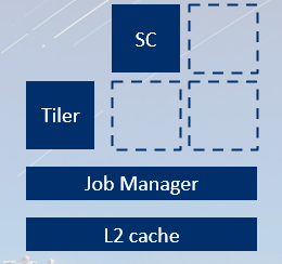
Midgard 架构详解
架构革新
| 特性 | 说明 |
|---|---|
| 统一着色器核心 | 一种核心处理所有着色任务 |
| Job Manager | 新增硬件调度单元,协调多核任务执行 |
| API 支持 | OpenGL ES 3.x、OpenCL |
 |
关键优化技术
Constant Tile Elimination (CTE) —— 恒定 Tile 消除
原理:
- Tile 着色完成后,计算颜色的 CRC 哈希
- 与内存中现有颜色的哈希比较
- 哈希相同 → 跳过写回
适用场景:
- ❌ 对 3D 内容帮助有限
- ✅ UI 和 2D 游戏效果显著(屏幕大部分静态)
💡 帧缓冲带宽是简单内容的主要功耗来源,跳过写回可大幅省电
Forward Pixel Kill (FPK) —— 前向像素剔除
- 首次出现: Mali-T620(第二代 Midgard)
- 实现 隐藏面消除(Hidden Surface Removal)
- 避免对被遮挡像素执行无用着色
ASTC 纹理压缩
- 全称: Adaptive Scalable Texture Compression
- 由 ARM 设计,捐赠给 Khronos
- 成为 Vulkan / OpenGL ES / OpenGL 官方标准
AFBC —— ARM 帧缓冲压缩
| 版本 | 支持格式 | 压缩率 |
|---|---|---|
| 初代 | 仅 UNORM 数据类型 | 25%~50% |
| 后续 | 新增浮点格式支持 | - |
⚠️ 初代不支持浮点,无法用于 HDR 渲染
TRIP 架构(Midgard 算术核心)
设计理念
不是 Warp,而是 SIMD 向量设计:
- 每个线程看到 向量指令(类似 ARM NEON)
- 数据通路宽度:128-bit
vec4FP32vec8FP16
三类并行流水线
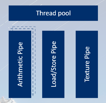
┌────────────────────────────────────────────────────────┐
│                      Shader Core                       │
│  ┌──────────────┐ ┌──────────────┐ ┌──────────────┐    │
│  │  Arithmetic  │ │  Load/Store  │ │   Texture    │    │
│  │     Pipe     │ │     Pipe     │ │     Pipe     │    │
│  │              │ │              │ │              │    │
│  │   All Math   │ │Memory Access │ │   Texture    │    │
│  │  Operations  │ │   Varying    │ │  Filtering   │    │
│  │              │ │Interpolation │ │              │    │
│  └──────────────┘ └──────────────┘ └──────────────┘    │
│          ↑               ↑                ↑            │
│          └───────────────┴────────────────┘            │
│           Three-Pipeline Parallel Execution            │
└────────────────────────────────────────────────────────┘
Shader 优化核心: 识别哪个管线是瓶颈
线程与寄存器权衡
| 配置 | 线程数 | 向量寄存器数 |
|---|---|---|
| 最大线程 | 256 | 4 |
| 最大寄存器 | 更少 | 更多 |
优化建议:
- Fragment Shader: 尽量使用 满线程数
- 原因:需要隐藏 内存延迟
- ARM 离线编译器可查看寄存器使用统计
Bifrost 架构革新
设计目标
- 追求 更高能效
- 支持更高核心数量
- 基础规格不变:16×16 Tile,1 texel/cycle,1 pixel/cycle
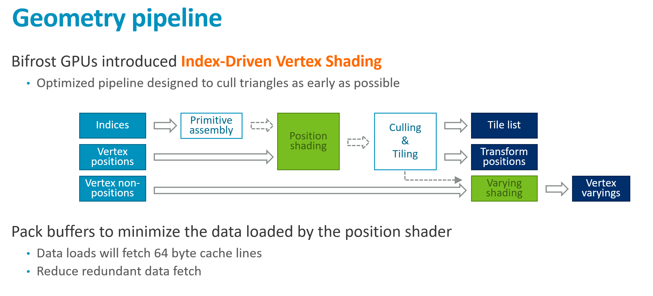
Index-Driven Vertex Shading(索引驱动顶点着色)
核心思想:将顶点着色拆分为两阶段
阶段1: 所有顶点 → 仅计算 Position
              ↓
        执行裁剪/剔除
              ↓
阶段2: 仅可见顶点 → 计算 Varyings
💡 避免为不可见顶点计算昂贵的 Varying 数据
新增浮点帧缓冲支持
- 对应 OpenGL ES 3.2 规范
- 支持 HDR 渲染 流程
Warp-Based 着色器架构
从 SIMD 到 Warp 的转变
| 特性 | Midgard (SIMD) | Bifrost (Warp) |
|---|---|---|
| 执行模型 | 向量指令/线程 | 标量指令/线程 |
| Warp 宽度 | - | 4 线程(窄 Warp) |
| 每线程视角 | 128-bit 向量 | 32-bit 标量 |
| FP16 处理 | vec8 | vec2 SIMD 打包在标量中 |
异步执行单元设计
┌────────────────────────────────────────────────────────┐
│                 Execution Engine (EE)                  │
│  ┌──────────────────────────────────────────────────┐  │
│  │            • Executes Shader Programs            │  │
│  │            • Contains Arithmetic Pipe            │  │
│  │          • Issues Load/Texture Requests          │  │
│  └───────────────────────┬──────────────────────────┘  │
│                          │ Async Messages              │
│              ┌───────────┴───────────┐                 │
│              ▼                       ▼                 │
│      ┌──────────────┐         ┌──────────────┐         │
│      │ Texture Unit │         │  Load Unit   │         │
│      │   (Async)    │         │   (Async)    │         │
│      └──────────────┘         └──────────────┘         │
│              │                       │                 │
│              └───────────┬───────────┘                 │
│                          ▼                             │
│                 Returns Data Later                     │
└────────────────────────────────────────────────────────┘
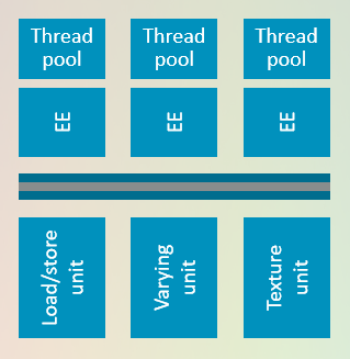
类似 Web 服务器 的请求-响应模型
资源配置对比
| 指标 | Midgard | Bifrost Gen1 |
|---|---|---|
| 峰值线程数 | 256 | 更高 |
| 寄存器 | 4-N 个 128-bit 向量 | 32 个标量(≈2x 容量) |
| 每周期操作数 | 42 | 24 |
为什么操作数下降但性能上升?
- SIMD 模型中存在 大量空闲通道
- Warp 模型更容易 发现并行执行机会
- 实际利用率显著提升
Bifrost 第二代
架构调整
- 将 两个旧着色器核心合并
- 因子化共享硬件,减少冗余
- 提升单核算力与效率
关键术语速查
| 术语 | 含义 |
|---|---|
| Fill Rate | 每秒可填充的像素数量 |
| Triangle Rate | 每秒可处理的三角形数量 |
| CTE | Constant Tile Elimination,跳过未变化 Tile 的写回 |
| FPK | Forward Pixel Kill,前向剔除被遮挡像素 |
| ASTC | 自适应可缩放纹理压缩格式 |
| AFBC | ARM 帧缓冲无损压缩 |
| Warp | 一组同步执行相同指令的线程 |
| IDVS | Index-Driven Vertex Shading,索引驱动顶点着色 |
Bifrost 与 Valhall 深度解析
Bifrost 架构核心变化
Shader Core 规格翻倍
| 参数 | Midgard | Bifrost |
|---|---|---|
| Tile 尺寸 | 16×16 | 16×16(不变) |
| 双线性采样/周期 | 1 | 2 |
| 混合像素/周期 | 1 | 2 |
| Warp 宽度 | 128-bit(4线程) | 256-bit(8线程) |
设计哲学:硬件融合
Bifrost "双核融合" 策略
[旧Core A] + [旧Core B]  →  [新大Core]
 • 公共硬件单元分摊(factorize)
 • 更宽数据通路 = 更高效
 • 结果:能效提升 25-30% 面积效率提升 25-30%
新增特性
| 特性 | 说明 |
|---|---|
| 各向异性过滤(Anisotropic Filtering) | 硬件原生支持 |
| 快速 YUV 采样 | 多媒体表面处理加速 |
| 改进的帧缓冲压缩 | 更好的 Vulkan 支持,内存视图(Memory View)与数据格式(Data Format) 正交化 |
Valhall 架构:当前主流(Galaxy S20+)
突破性变化:纹理与像素比例分离
首次打破 1:1 的纹理/像素比例:
| 能力 | 每周期每核心 |
|---|---|
| 双线性纹理采样 | 4 次 |
| 混合像素输出 | 2 次(不变) |
原因:
- 现代内容使用更复杂的纹理过滤(各向异性、三线性)
- 后处理 Shader 需要多次纹理采样
- 纹理需求增长快于像素输出需求
异步频率域
┌──────────────────────────────────────────────────────────────────────┐
│                 Valhall Dual Frequency Domain Design                 │
│                                                                      │
│  ┌─────────────────────────────┐    ┌─────────────────────────────┐  │
│  │         Shader Cores        │    │     Job Manager + Tiler     │  │
│  │ ─────────────────────────── │    │ ─────────────────────────── │  │
│  │ Low Frequency               │    │ High Frequency              │  │
│  │ • Highly Parallel           │    │ • Single Scheduler          │  │
│  │ • Low Voltage = Saves Power │    │ • Avoids Bottlenecks        │  │
│  └─────────────────────────────┘    └─────────────────────────────┘  │
└──────────────────────────────────────────────────────────────────────┘
新增硬件特性
| 特性 | 详情 |
|---|---|
| FP16 硬件混合 | 针对 FP16 目标的混合操作 不消耗 Shader Core 周期 |
| 帧缓冲压缩扩展 | 支持所有 32-bit/像素 格式 |
⚠️ 限制: RGB/RGBA FP16(64-bit)格式 仍无法压缩,未来硬件将支持
算术单元架构
三条并行流水线:
| 流水线 | 功能 | Warp 宽度 |
|---|---|---|
| FMA | 融合乘加(Fused Multiply-Accumulate) | 16-wide |
| CVT | 类型转换(Convert) | 16-wide |
| SFU | 特殊函数(sin/cos/log/exp/pow) | 4-wide(需4周期完成1个warp) |
其他改进:
- Warp 宽度再次翻倍:16 线程
- 线程数增加 → 更好的 延迟隐藏
- 寄存器数量保持不变
官方资源提示
📊 ARM 官网提供 Mali GPU 数据表(Mali-T700 及以上),包含:
- 各单元的速度与容量参数
- 寄存器数量
- 缓存大小
- 完整的硬件规格参考
移动端性能优化核心原则
优化思维转变
不是"让事情更快",而是:
| 优化方向 | 具体做法 |
|---|---|
| 消除冗余 | 移除相机外的 Draw Call、被遮挡物体 |
| 修正错误配置 | 不透明物体关闭混合 |
| 接受近似 | 图形不需要 bit-exact,5% 性能换"足够好"是划算的 |
💡 最快的优化往往是"移除"而非"改进"
性能差异规划
设备性能跨度:
| 设备类型 | 相对性能 |
|---|---|
| 低端手机 | 1x(基准) |
| 高端手机 | ~6x |
| 平板电脑 | ~10x(更大散热空间) |
⚠️ 如果计划跨设备发布同一款游戏,必须提前规划质量等级
帧率与分辨率:最关键的早期决策
填充率对比
| 配置 | 分辨率 | 帧率 | 填充率 |
|---|---|---|---|
| 低端目标 | 720p | 30 fps | ~30 MP/s |
| 高端目标 | 1440p | 90 fps | ~340 MP/s |
差距:超过 10 倍!
移动端现实挑战
- 屏幕分辨率:1440p 甚至更高
- 色彩空间:Wide Color Gamut(P3)
- 刷新率:90 Hz / 120 Hz
推荐策略
┌────────────────────────────────────────────────────────┐
│          Framerate/Resolution Decision Matrix          │
│                                                        │
│    Default Baseline: 1080p @ 60 fps                    │
│          ↗                        ↘                    │
│    High-End Devices:         Low-End Devices:          │
│    Consider Upgrading        Consider Downgrading      │
│                                                        │
│    Caution! These factors are Multiplicative!!!        │
│    • Framerate ×2    → Budget ÷2                       │
│    • Resolution ×2   → Budget ÷2                       │
│    • Both Combined   → Budget ÷4                       │
└────────────────────────────────────────────────────────┘
HDR 与颜色格式的代价
HDR 的隐藏成本
| 影响 | 说明 |
|---|---|
| 帧缓冲体积 | 翻倍(FP16 vs UNORM8) |
| Mali 帧缓冲压缩 | ❌ 不可用 |
| Display Controller 压缩 | ❌ 可能也不可用 |
决策建议
⚠️ 颜色格式是 乘法因子 —— 每一帧、每一像素都会叠加这个成本
在追求"新潮技术"前,务必评估 实际画质收益 与 性能代价
资源预算与帧构建
高分辨率帧缓冲的带宽代价
带宽爆炸示例
以 RGBA FP16 @ 1440p @ 90fps 为例:
| 组件 | 带宽消耗 |
|---|---|
| 单个表面 | >2.5 GB/s |
| + 显示控制器回读 | ~5 GB/s |
| 仅显示更新的功耗 | ~0.5W(GPU还未工作) |
⚠️ 分辨率 × 格式 × 帧率 三者相乘,数值增长极快
资产预算规划
Draw Call 预算
| 平台 | 建议预算 |
|---|---|
| 通用移动端 | ~500 Draw Calls/帧 |
| 高端设备 | 可适当超出 |
| 入门级设备 | 更需严格控制 |
原因:
- Draw Call 是 驱动最昂贵的操作
- 入门机型可能仅有 8 个小核心 CPU
- CPU 花在 Draw Call 上 = 无法用于渲染
几何预算
TBR 的痛点: 几何数据必须写回内存
需要严格控制:
- 图元数量(Primitive Count)
- 顶点复杂度
- 入门设备可能仅有 512MB RAM
纹理预算
- 材质层数、分辨率、压缩格式
- GPU 纹理处理能力通常充足
- 主要瓶颈: 内存占用与分发包大小
Shader 周期预算计算
预算公式
实例计算
配置: Mali-G72 双核 @ 700MHz,目标 1080p@60fps
实际可用: ~9.5 周期(考虑利用率损失)
预算分配
11 周期必须覆盖所有操作:
• 顶点着色
• 片段着色
• 后处理
• 显示合成回退(如有)
预算不足时的策略
| 策略 | 示例 |
|---|---|
| 降级效果 | 低端设备禁用后处理 |
| 降帧率 | 60fps → 30fps(预算翻倍) |
| 降分辨率 | 1080p → 720p |
| 混合分辨率 | 主画面1080p,后处理720p叠加 |
高端设备注意事项
- 性能充裕,真正挑战是功耗管理
- 无硬性周期限制
- 关注 CPU + 内存 + Shader 的综合负载
帧构建:TBR 优化的核心
优化优先级
先确保帧骨架正确,再做细节优化
核心要素:
- Render Pass 划分
- Compute Dispatch 调度
- 数据流向(DRAM 访问模式)
Tile Memory:TBR 的超能力
┌───────────────────────────────────────────────────────────┐
│                 Tile-Based Rendering Flow                 │
│                                                           │
│  [DRAM]  ──Load──>  [Tile Memory]  ──Store──>  [DRAM]     │
│    ↑                      ↑                      ↑        │
│ Expensive!     All intermediate states       Expensive!   │
│                  (Zero DRAM access)                       │
└───────────────────────────────────────────────────────────┘
TBR 的代价与收益:
| 代价 | 收益 |
|---|---|
| 额外的三角形带宽 | Tile 内渲染零带宽 |
⚠️ 如果用不好 Tile Memory,代价照付但无收益 → 最差结果
Tile Memory 生命周期
| 阶段 | 行为 |
|---|---|
| Pass 开始 | Clear → 无需加载;否则从 DRAM Load |
| Pass 中间 | 所有操作在 Tile 内完成 |
| Pass 结束 | Store 或 Resolve(MSAA)回 DRAM |
Vulkan 的优势
Vulkan 中 Render Pass 是 显式 API 构造 :
// Vulkan Render Pass 配置
VkAttachmentDescription attachment = {
    .loadOp  = VK_ATTACHMENT_LOAD_OP_CLEAR,    // 明确 Load 操作
    .storeOp = VK_ATTACHMENT_STORE_OP_STORE,   // 明确 Store 操作
    // 或 DONT_CARE 可跳过
};
Load/Store Op 选项:
| 操作 | 说明 |
|---|---|
| LOAD | 从 DRAM 读取(昂贵) |
| CLEAR | 直接清零(便宜) |
| DONT_CARE | 内容不重要,可跳过 |
| STORE | 写回 DRAM(昂贵) |
| RESOLVE | MSAA 解析后写回 |
关键优化原则速查
| 原则 | 操作 |
|---|---|
| 最小化 DRAM 访问 | 减少 Load/Store 次数 |
| 善用 Clear | 避免不必要的 Load |
| 合并 Render Pass | 减少中间写出 |
| 关注格式大小 | FP16 带宽 = RGBA8 的两倍 |
| 预算先行 | 计算周期/像素预算再设计效果 |
Render Pass 与数据流优化
Vulkan Render Pass 操作详解
Load 操作
| Load Op | 行为 | 性能 |
|---|---|---|
| VK_ATTACHMENT_LOAD_OP_LOAD | 从内存加载现有内容 | 消耗带宽 |
| VK_ATTACHMENT_LOAD_OP_CLEAR | 固定功能硬件初始化为清除色 | 几乎免费 ✅ |
| VK_ATTACHMENT_LOAD_OP_DONT_CARE | 不关心初始值 | 几乎免费 ✅ |
Store 操作
| Store Op | 行为 | 性能 |
|---|---|---|
| VK_ATTACHMENT_STORE_OP_STORE | 写回内存 | 消耗带宽 |
| VK_ATTACHMENT_STORE_OP_DONT_CARE | 丢弃数据 | 零成本 ✅ |
Vulkan 清除与解析的正确姿势
清除(Clear)
| 方式 | 实现 | 推荐度 |
|---|---|---|
| Load Op Clear | 固定功能硬件 | ✅ 始终使用 |
| vkCmdClear | 生成全屏 Shader Quad | ❌ 避免 |
💡 Pass 开始时的清除 必须 用 Load Op
MSAA 解析(Resolve)
┌─────────────────────────────────────────────────────────────────┐
│  CORRECT: Render Pass Resolve Attachment                        │
│                                                                 │
│  [Tile Memory]  ──Resolve + Store──>  [Single-Sample Target]    │
│        ↓                                                        │
│  [MSAA Data]    ──Store DONT_CARE──>  (Discard)                 │
│                                                                 │
│  • Multi-sample data never leaves the GPU                       │
│  • Resolve is done inline as part of the Tile write-back        │
└─────────────────────────────────────────────────────────────────┘

┌─────────────────────────────────────────────────────────────────┐
│  WRONG: vkCmdResolveImage                                       │
│                                                                 │
│  [Tile] ──Store──> [DRAM MSAA Data] ──Load──> [GPU] ──Resolve──>│
│                                                                 │
│  • MSAA data written to memory (huge and incompressible)        │
│  • Read back into GPU for resolving                             │
│  • Bandwidth cost is CATASTROPHIC                               │
└─────────────────────────────────────────────────────────────────┘
OpenGL ES Render Pass 管理
Pass 边界识别
OpenGL ES 没有显式 Render Pass ,驱动根据行为推断:
| 触发新 Pass 的操作 | 说明 |
|---|---|
glBindFramebuffer() | 绑定新 FBO |
eglSwapBuffers() | 窗口表面刷新 |
glFlush() / glFinish() | ⚠️ 强制分割 |
| 中途修改 Attachments | ⚠️ 强制分割 |
FBO 最佳实践
FBO 黄金法则
1. 每种状态组合 → 独立 FBO
2. 设置一次 Attachments,永不修改
3. D24S8 格式 → 同时绑定深度和模板(配合帧缓冲压缩)
模拟 Load/Store Op
| Vulkan 等效 | OpenGL ES 实现 |
|---|---|
| Load Clear | glClear() 作为 Pass 第一个操作 |
| Load Don't Care | glInvalidateFramebuffer() 作为 Pass 第一个操作 |
| Store Don't Care | glInvalidateFramebuffer() 作为 Pass 最后操作 |
⚠️ 如果先画东西再 Clear,会变成 Clear Quad Shader ,成本高昂
MSAA 解析
| 方式 | 推荐度 |
|---|---|
glBlitFramebuffer() | ❌ 写回再读取 |
| EXT_multisampled_render_to_texture | ✅ Tile 写回时内联解析 |
💡 该扩展所有移动端厂商都支持,是移动 MSAA 的首选
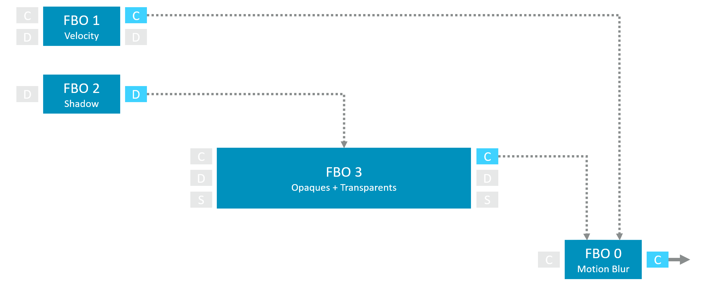
帧图(Frame Graph)分析方法
帧图元素
帧图符号说明
节点:FBO / Render Pass
小方块:Attachments(Color/Depth/Stencil)
实线 ── Attachment 直接传递
虚线 ── 作为纹理采样
示例帧图
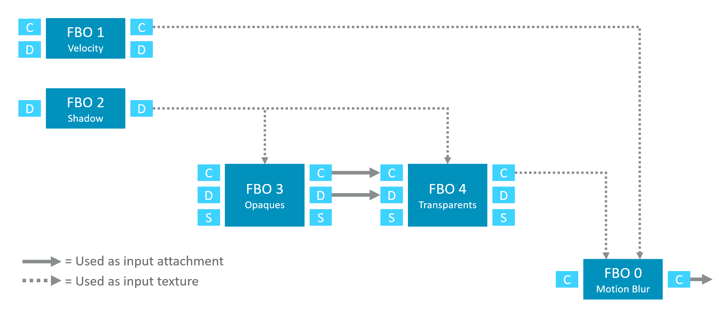
帧图优化原则
| 情况 | 优化操作 | 收益 |
|---|---|---|
| 无数据来源的输入 | 使用 Clear / Don't Care | 避免冗余读取 |
| 无数据消费的输出 | 使用 Invalidate / Don't Care | 避免冗余写入 |
| Pass 间直接传递 | 保持 Attachment 不变 | 可能合并或优化 |
关键洞察:
总结:帧构建检查清单
✅ Pass 开始:Clear 或 Don't Care(除非真正需要加载)
✅ Pass 结束:Invalidate 不再需要的 Attachments
✅ MSAA:使用 Resolve Attachment,永不 Blit/CmdResolve
✅ OpenGL ES:Clear 第一、Invalidate 最后
✅ FBO:一次构建,永不修改
✅ 画帧图:可视化数据流,消除冗余读写
Render Pass 合并与延迟着色优化
Render Pass 合并优化
核心原则
当两个 Attachment 仅被后续 Pass 直接消费,而非作为纹理读取时,可以合并为单个 Pass
┌────────────────────────────────────────────────────────────────┐
│  BEFORE MERGING: Bandwidth Waste                               │
│                                                                │
│  [Pass 1: 3D Render] ──Store──> [DRAM] ──Load──> [Pass 2: UI]  │
│                                                                │
│  AFTER MERGING: Zero Intermediate Bandwidth                    │
│                                                                │
│  [Single Pass: 3D Render + UI Overlay]                         │
│        ↓                                                       │
│  Data stays entirely inside Tile Memory                        │
└────────────────────────────────────────────────────────────────┘
最常见场景
| 场景 | 问题 | 解决方案 |
|---|---|---|
| 3D + UI 分离 | 子系统交接导致 Pass 分割 | 将 UI 叠加追加到同一 Pass |
| 多阶段后处理 | 每阶段独立 Pass | 尽可能合并为连续 Draw |
💡 这是游戏中 最常见的优化机会
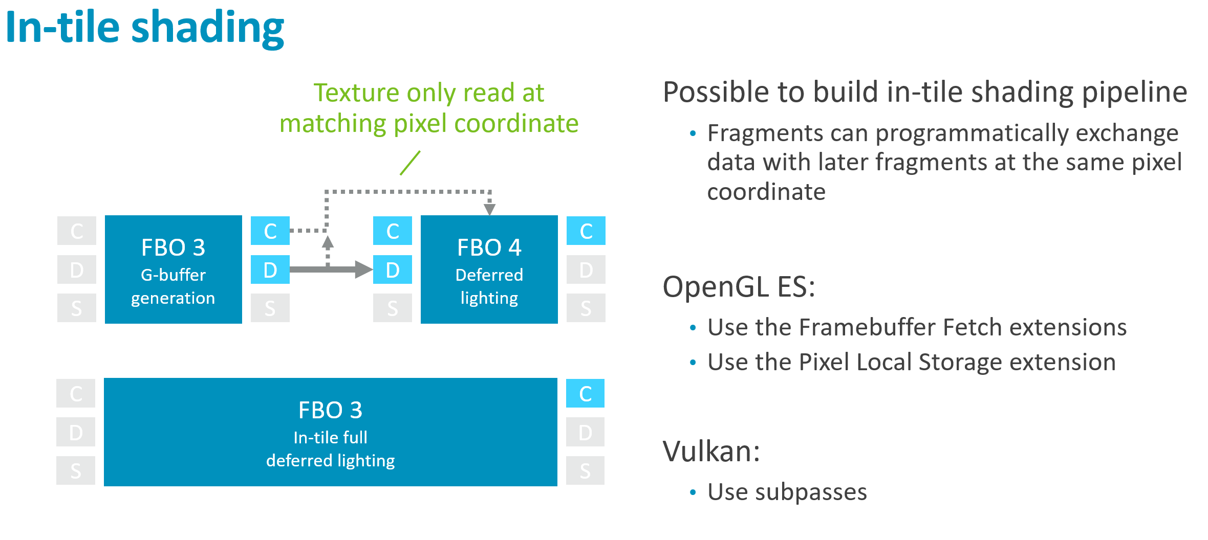
延迟着色的 In-Tile 优化
特殊模式:同像素坐标读取
前提条件:
- G-Buffer 数据仅在 相同像素坐标 被读取
- 无跨 Tile 内存访问
- 应用程序能 算法层面保证 这一点
In-Tile 延迟着色管线
┌────────────────────────────────────────────────┐
│  Traditional vs. In-Tile Deferred Pipeline     │
│                                                │
│  Traditional (DRAM Heavy):                     │
│  [Geometry] ──Write G-Buffer──> [DRAM]         │
│                                   ↓            │
│            [Lighting] <──Read G-Buffer         │
│                                                │
│  In-Tile TBDR (Zero G-Buffer Bandwidth):       │
│  ┌──────────────────────────────────────────┐  │
│  │        Single Merged Render Pass         │  │
│  │                                          │  │
│  │ [Geometry]   → Write G-Buffer to Tile Mem│  │
│  │      ↓                                   │  │
│  │ [Lighting]   ← Read local Tile Mem data  │  │
│  │      ↓                                   │  │
│  │ [Accumulate] → Update Tile Mem result    │  │
│  │      ↓                                   │  │
│  │ [End Pass]   → Discard G-Buffer DONT_CARE│  │
│  └──────────────────────────────────────────┘  │
│                                                │
│      G-Buffer is NEVER written to DRAM         │
└────────────────────────────────────────────────┘
API 实现方式
| API | 机制 |
|---|---|
| Vulkan | Subpasses + Input Attachments |
| OpenGL ES | EXT_shader_pixel_local_storage / EXT_shader_framebuffer_fetch |
Mali 上的性能权衡
带宽 vs 性能
| 方面 | 影响 |
|---|---|
| 带宽 | ✅ 必定节省 —— 数据保证在 Tile 内 |
| 性能 | ⚠️ 可能略有损失 |
性能损失原因:
- Tile Memory 数据流存在 数据依赖
- Shader Core 指令调度需要管理这些依赖
- 可能产生 局部气泡(Bubbles)
推荐策略
| 场景 | 建议 |
|---|---|
| 热限制(Thermally Bound)的高端Content | ✅ 强烈推荐 —— 能耗节省显著 |
| 性能受限场景 | 需实测权衡 |
功耗预算实例分析
G-Buffer 带宽成本
配置: 1080p G-Buffer @ 60fps(含帧缓冲压缩)
| 指标 | 数值 |
|---|---|
| G-Buffer 带宽功耗 | ~200mW |
| 典型 GPU 功耗预算 | 1.5W |
| CPU + 内存预算 | ~1W |
| G-Buffer 占比 | 15-20% 总功耗预算 |
关键要点总结
| 优化类型 | 收益 | 实现难度 |
|---|---|---|
| Pass 合并(相邻子系统) | 高 | 低 |
| In-Tile 延迟着色 | 极高(带宽归零) | 中 |
| Subpass 替代独立 Pass | 高 | 需 API 适配 |
💡 帧构建优化是 TBR 优化的第一优先级 —— 先修骨架,再调细节
帧图分析与压缩优化
帧图(Frame Graph)可视化分析
帧图的威力
绘制帧图本身就是强大的优化工具 —— 通过可视化 Render Pass 之间的数据流,优化机会一目了然
常见优化模式识别
| 模式 | 特征 | 优化方案 |
|---|---|---|
| 孤立 Pass | 输出无人消费 | 本帧直接跳过提交 |
| 缺失 Invalidate | 深度附件写后未标记丢弃 | 添加 DONT_CARE Store Op |
| Feed-through | 唯一消费者是下一个 Pass | 合并 Pass |
实战案例
┌───────────────────────────────────────────────┐
│  BEFORE: 8-9 Passes Exchanging Data           │
│                                               │
│  [Pass A] ──Depth+Stencil+Color──> [Pass B]   │
│                       ↓                       │
│               All Read/Write at 1080p         │
│                                               │
│  AFTER: Merged Feed-Through Passes            │
│                                               │
│  SAVED: 60 MB/frame Bandwidth                 │
│  Visual Difference: Zero                      │
└───────────────────────────────────────────────┘
💡 关键洞察: 这纯粹是数据流优化,渲染结果完全相同
AFBC 帧缓冲压缩详解
基本特性
| 属性 | 说明 |
|---|---|
| 压缩类型 | 无损压缩 |
| 应用介入 | 无需 Opt-in,自动启用 |
| 典型带宽节省 | 30-50%(依赖图像内容) |
硬件代际限制
| 硬件代 | 支持格式 |
|---|---|
| Valhall | ≤32-bit/像素格式 |
| Midgard / Bifrost | 仅 UNORM 格式 |
不支持的格式:
- ❌ HDR RGB / RGBA FP16
- ❌ Float / Int / Signed Int(旧硬件)
- ❌ 多采样数据(写回内存时)
⚠️ MSAA 数据写回内存 = 全额带宽成本,必须 In-Tile Resolve
运行时使用限制
AFBC 仅在特定路径生效:
	✅ Frame Buffer 写入路径
	✅ Texturing 读取路径
	❌ Image Load/Store(Compute Shader)

首次 Image 使用 → 触发解压 Pass → 性能损失
驱动随后标记纹理 → 永久禁用压缩
Bifrost 特定约束
For Vulkan, use of AFBC is determined statically based on the image flags used when the image view is created.
To use AFBC, images must use IMAGE_TILING_OPTIMAL memory layout, and must not use IMAGE_USAGE_STORAGE, IMAGE_USAGE_TRANSIENT, or IMAGE_CREATE_ALIAS.
| 要求 | 说明 |
|---|---|
| Image Tiling | 必须为 VK_IMAGE_TILING_OPTIMAL |
| Storage | ❌ 不可用 |
| Transient | ❌ 不可用 |
| Memory Aliasing | ❌ 不支持(压缩与格式绑定) |
Tile Memory 容量管理
设计规格
| 硬件代 | 每像素颜色预算 |
|---|---|
| 旧硬件(Midgard/Bifrost) | 128 bits/pixel |
| 新硬件(Valhall Gen2) | 256 bits/pixel |
深度和模板缓冲 独立分配 ,不占用颜色预算
超出预算时的 Tile 降级
Using more than 256 bits per pixel on a modern Mali will result in the tile size dropping, which will incur efficiency overheads.
预算超出 → Tile 尺寸递减:

16×16 → 16×8 → 8×8 → 8×4 → 4×4

影响因素:
• 颜色格式位深
• 多采样级别
• MRT 附件数量
预算消耗示例
| 配置 | 每像素消耗 | 状态 |
|---|---|---|
| RGBA8 × 1 | 32 bits | ✅ 充裕 |
| RGBA8 × 4 MRT | 128 bits | ⚠️ 旧硬件极限 |
| RGBA16F × 2 + 4xMSAA | 256+ bits | ❌ 可能降级 |
⚠️ HDR + G-Buffer 或 HDR + MSAA 很容易超出预算
Compute Shader 使用指南
核心建议
将 Compute Dispatch 纳入帧图管理 —— 它本质上就是一种 Render Pass
Compute vs Fragment 对比
| 方面 | Compute Shader | Fragment Shader |
|---|---|---|
| AFBC 压缩 | ❌ 不可用 | ✅ 自动启用 |
| Image Load/Store | 较慢 | 使用 Texturing(更快) |
| 固定功能硬件 | ❌ 无法使用 | ✅ 插值器等可用 |
| 灵活性 | 打破固定功能沙箱 | 受限于光栅化管线 |
何时使用 Compute
| 场景 | 推荐度 |
|---|---|
| 1:1 替换 Fragment | ❌ 通常更慢 |
| 跨像素共享计算 | ✅ |
| 非光栅化算法 | ✅ |
| 工作组内数据共享 | ✅ |
💡 原则: 使用 Compute 必须有 算法层面的理由 ,而非单纯替换
同步、依赖与缓冲策略
Compute Shader 的正确认知
打破迷信
⚠️ Compute Shader 不是魔法 —— 不会仅因"是 Compute"就自动更快
真正的优势来源:
- 将多个片段合并为单个 Work Item
- 更灵活地利用并行性
- 自定义内存访问模式
管线同步:避免阻塞
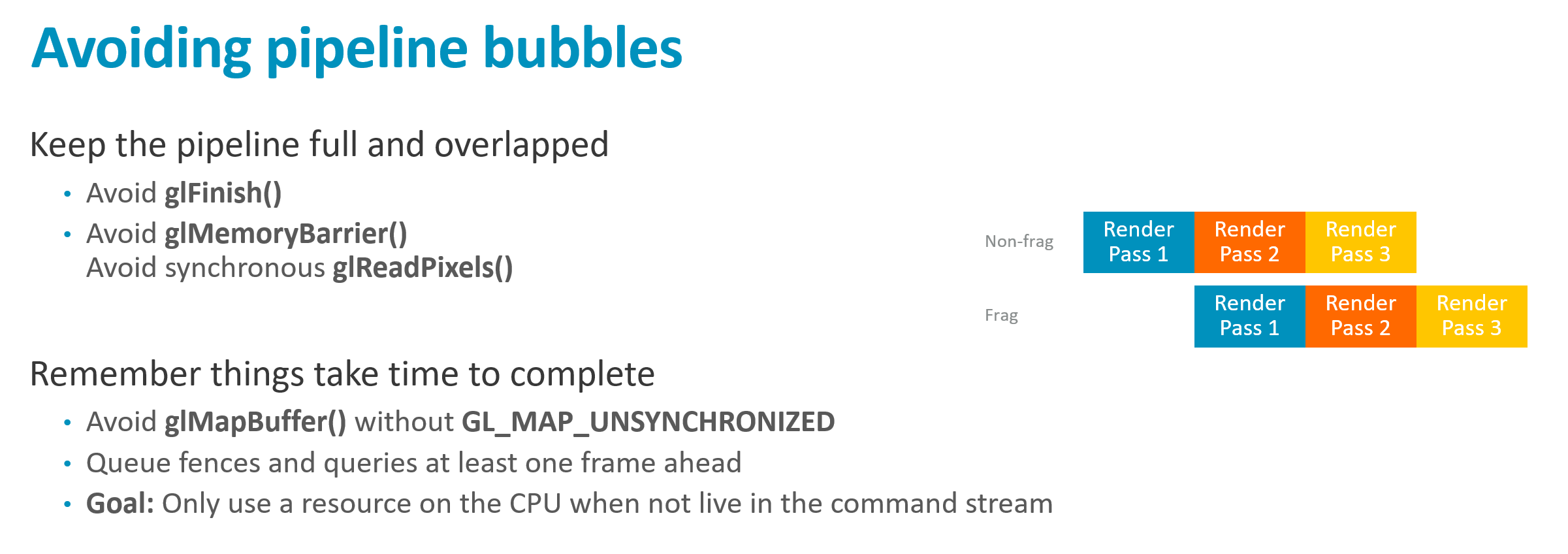
危险操作清单
| 危险调用 | 问题 |
|---|---|
glFinish | 强制 CPU 等待 GPU 完成 |
glMemoryBarrier | 可能导致过度同步 |
glReadPixels | 回读阻塞 |
glMapBuffer(无 GL_MAP_UNSYNCHRONIZED) | 隐式同步 |
延迟感知
关键数字: 管线延迟通常 ≥1 帧
Query / Fence 使用策略

❌ 错误:提交后立即等待
   → 阻塞等待结果 → 管线排空

✅ 正确:提前 1-2 帧发起查询
   → 激进流水线化 → 结果就绪时再读取
💡 OpenGL ES 驱动通常自动处理得很好,问题 API 众所周知
Vulkan 依赖管理:头号性能杀手
问题本质
这是 Vulkan 应用中最常见的性能问题:依赖设置过于保守
错误示例
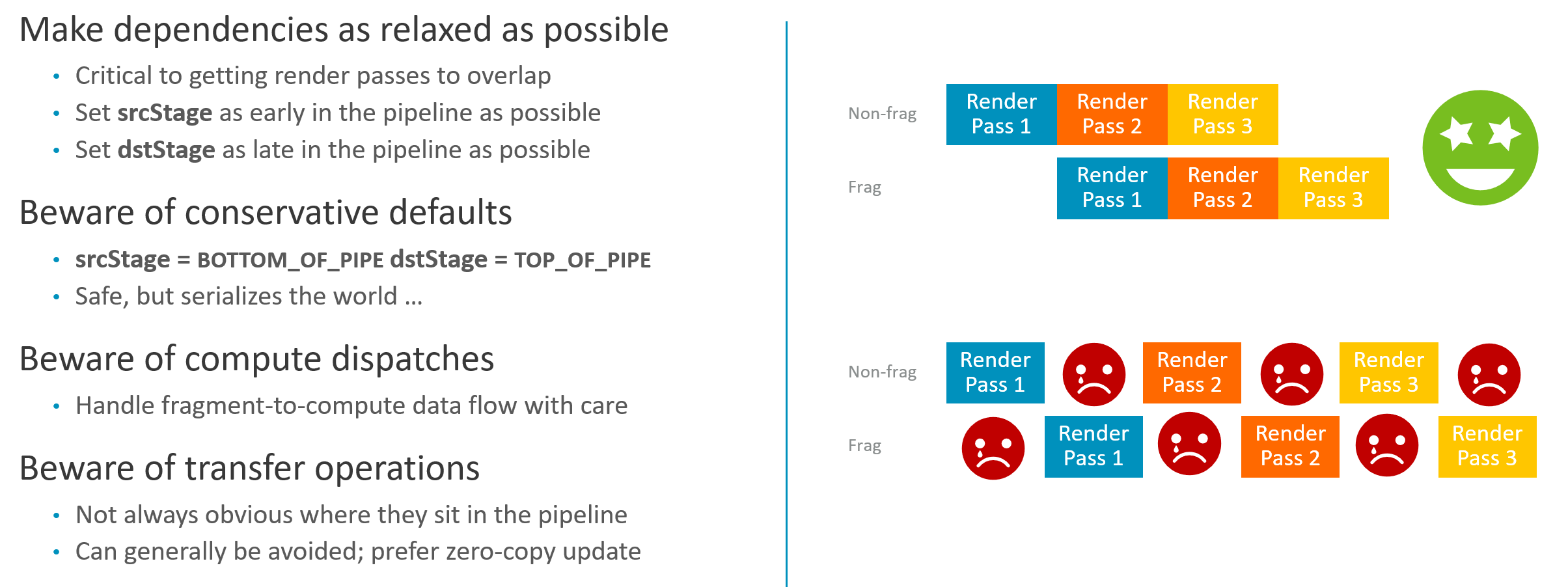
❌ 过度保守的依赖
srcStageMask = VK_PIPELINE_STAGE_BOTTOM_OF_PIPE_BIT
dstStageMask = VK_PIPELINE_STAGE_TOP_OF_PIPE_BIT
含义:"前一个 Pass 完全结束后,下一个 Pass 才能开始"
结果:完全串行化,零重叠
正确做法
| 原则 | 说明 |
|---|---|
| srcStage 尽早设置 | 数据何时产出就设何时 |
| dstStage 精确匹配 | 实际消费阶段是什么就设什么 |
示例:
数据由顶点着色器产出 → srcStage = VERTEX_SHADER
数据被片段着色器消费 → dstStage = FRAGMENT_SHADER

✅ 允许后续 Pass 的顶点阶段与前一 Pass 重叠执行
Mali Compute 调度特性
槽位架构
Mali 双槽位调度
[Non-Fragment 槽]  ←── Vertex + Compute
       ↓
[Fragment 槽]      ←── Fragment Shading
正常数据流:Non-Fragment → Fragment(下游)
逆向依赖问题
Fragment → Compute 的数据流(逆向)

   调度上是"向上"依赖,可能导致轻微卡顿
缓解策略:
- 在 Compute Shader 前后放置 非依赖工作
- 给调度器提供 气泡容量 来重新排布
移动端 Transfer Ops 优化
桌面 vs 移动
| 平台 | 内存架构 | Transfer Ops |
|---|---|---|
| 桌面 | 系统 RAM + 独显 VRAM(PCIe) | 必需 |
| 移动 | 统一内存 | 大多可省略 |
💡 移动端 CPU/GPU 共享同一内存池 → 直接上传,GPU 即可见
Swap Chain 缓冲策略
双缓冲 + VSync 的困境
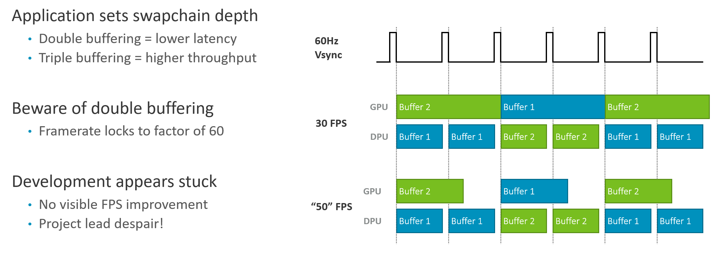
┌─────────────────────────────────────────────────────────────┐
│ SCENARIO: GPU@50fps, Display@60Hz, Double Buffering + VSync │
│                                                             │
│ TIMELINE:                                                   │
│   ┌────────┬────────┬────────┬────────┐                     │
│   │ V-Sync1│ V-Sync2│ V-Sync3│ V-Sync4│  Display @ 60Hz     │
│   └────────┴────────┴────────┴────────┘                     │
│   │←─ Buf1 ──→│←─ Buf1 ──→│←─ Buf2 ──→│  Screen Output      │
│               ↑                                             │
│         Buf2 not ready, Buf1 re-scanned (Missed V-Sync)     │
│                                                             │
│ GPU finishes Buf2 → No back buffer available → STALL        │
│ EFFECTIVE FPS: 30 fps (due to 60/2 quantization)            │
└─────────────────────────────────────────────────────────────┘
三缓冲的权衡
| 方面 | 双缓冲 | 三缓冲 |
|---|---|---|
| 吞吐量 | 受限于 VSync 对齐 | ✅ GPU 始终有 Buffer 可渲染 |
| 输入延迟 | 较低 | ⚠️ +1 帧延迟 |
| 触控手感 | 更灵敏 | 略显迟钝 |
三缓冲:引入"草稿缓冲区"
→ GPU 永不闲置
→ 帧率 50fps → 实际 50fps
→ 代价:最坏情况延迟增加一帧
帧缓冲策略与游戏引擎实践
帧缓冲策略选择
双缓冲 vs 三缓冲
| 配置 | 适用场景 | 特性 |
|---|---|---|
| 双缓冲 + VSync | 发布版本 | 降低输入延迟,FPS 游戏尤为重要 |
| 三缓冲 / 禁用 VSync | 开发阶段 | 测量真实性能,无帧率锁定 |
⚠️ 开发时禁用 VSync,发布前 务必恢复
移动端屏幕旋转陷阱
物理扫描方向
大多数移动屏幕:竖屏扫描
┌─────┐
│  ↓  │  扫描线沿短边方向
│  ↓  │  硬件固定,无法改变
│  ↓  │
└─────┘
灾难场景:内存布局与扫描方向不匹配
| 情况 | 性能影响 |
|---|---|
| App 布局与扫描方向一致 | 显示控制器直接输出 ✅ |
| App 布局与扫描方向垂直(差90°) | 显示控制器回退到 GPU ❌ |
Pre-Transform 处理
| API | 处理方式 |
|---|---|
| OpenGL ES | 驱动自动与 OS 协商变换 |
| Vulkan | 应用程序显式管理 |
Vulkan 正确流程:
1. 获取新 Swap Chain 时检查 pre-transform hint
2. 设备旋转 → OS 更新 hint
3. 应用重建 Swap Chain 并应用 transform
4. 插入几何变换旋转/翻转渲染
5. 显示控制器无需额外工作
游戏引擎宏观优化
Draw Call 削减策略
| 策略 | 说明 |
|---|---|
| 静态批处理 | 离线合并物体 |
| 动态批处理 | 运行时合并 |
| 实例化绘制 | glDrawInstanced |
| CPU 剔除 | 利用场景知识提前剔除 |
CPU 剔除的不可替代性
GPU 无法做到的剔除:
• 整个物体在相机后方
• 整个房间因门不可见而隐藏
原因:GPU 必须先完成顶点着色才知道位置
      → 几何已被处理 → 带宽/周期已消耗
状态变更优化
- 按状态排序 Draw Call → 最小化状态切换次数
- 显著降低 Draw Call 成本
多线程与 Vulkan 优势
能效公式
Vulkan 的 CPU 端革新
| 特性 | 收益 |
|---|---|
| 更显式 | Draw Call 更廉价 |
| 设计支持多线程 | 并行构建 Command Buffer |
| 驱动状态追踪更少 | 异步模型匹配硬件 |
💡 GPU 负载不会剧变(硬件相同),但 CPU 负载可显著降低
随机帧卡顿诊断
典型症状
正常运行 60fps → 突然掉到 30/20fps → 恢复
常见原因:资源上传与修改
| 问题 | 机制 |
|---|---|
| 游戏中上传大纹理/缓冲 | 占用带宽,阻塞管线 |
| 修改仍被引用的资源 | 触发 Copy-on-Write / Resource Ghosting |
Copy-on-Write 机制详解
场景:纹理仍被排队中的 Draw Call 引用

此时尝试修改该纹理 →

驱动选择:
A) 阻塞整个管线等待引用释放 → 严重卡顿
B) 创建纹理副本 + 应用修改 → 内存分配 + 数据拷贝
两者都很昂贵!
解决方案
| 策略 | 说明 |
|---|---|
| 关卡加载时完成 | 将资源上传移出游戏循环 |
| 避免修改活跃资源 | 等待引用释放再操作 |
| 多缓冲资源 | 轮换使用多个副本 |
 |
着色器编译、绘制策略与几何优化
着色器编译成本
编译与链接的真实代价
| 阶段 | 操作 | 耗时 |
|---|---|---|
| Compile | 生成 IR + 部分优化 | 慢(数十毫秒) |
| Link | 完整管线优化 + 代码生成 | 同样慢 |
⚠️ 常见误解:认为 Compile 慢但 Link 快 —— 两者都很慢
原因: 完整代码生成在 Link 阶段完成,整个管线一起优化
加速加载策略
- 跨运行缓存程序 → 避免每次启动都重新编译
- 使用
glGetProgramBinary/VkPipelineCache
绘制调度最佳实践
绘制顺序优化
| 类型 | 顺序 | 原因 |
|---|---|---|
| 不透明物体 | 前到后 | 最大化 Early-ZS 剔除 |
| 透明物体 | 后到前 | 正确混合 |
Mali 有 Hidden Surface Removal(HSR)

• 可应对后到前不透明绘制
• 但 Early-ZS 保证更彻底
• HSR 无法移除所有冗余

建议:前到后排序有帮助,但别花太多 CPU 做完美排序
干净的渲染状态设置
| 设置 | 建议 |
|---|---|
| 背面剔除 | 3D 绘制 始终开启 |
| 混合 | Alpha = 1 时 禁用 |
| Alpha to Coverage | 不需要时 禁用 |
⚠️ 即使状态"实际不生效",硬件无法预知 → 禁用多项优化
UI 渲染中的深度/模板清除
场景:每个 UI Widget 间清除深度/模板
❌ 全屏清除 → 成本不低
✅ 使用 Scissor 限制清除范围 → 最小化 Mid-pass Clear
Depth Pre-pass 在 Tile-Based 渲染器上的陷阱
双倍几何提交
Depth Pre-pass 工作流:

Pass 1: 几何 → 仅填充深度缓冲
Pass 2: 几何 → 使用深度进行着色

问题:几何提交两次 → 带宽翻倍写回主内存
与 HSR 功能重叠
- Depth Pre-pass 目的:避免重复着色
- HSR 已在做类似的事
- 实测案例:关闭 Depth Pre-pass 后游戏更快
💡 可以尝试,但要实测验证收益
OpenGL ES vs Vulkan 市场现状
当前格局
| 事实 | 说明 |
|---|---|
| 大多数开发中游戏 | 仍使用 OpenGL ES |
| 新游戏 | 许多仍选择 OpenGL ES |
OpenGL ES 占主导的原因
- 设备覆盖 —— 2-3 年前设备仅支持 OpenGL ES
- 早期 Vulkan 驱动 —— 稳定性/性能不佳
- 引擎支持成熟度 —— 最新引擎版本 Vulkan 才真正达到同等水平
- 工作室保守 —— 使用 18 个月前版本引擎开发
未来趋势
Vulkan 必然普及,但新项目采用预计还需 12-18 个月
几何内容优化
核心原则
GPU 是数据驱动处理器 —— 美术资产才是最大问题源
顶点优化策略
| 策略 | 说明 |
|---|---|
| 减少三角形数量 | 根本性优化 |
| 提高顶点复用 | 共享顶点跨三角形 |
| 减小每顶点字节数 | 数据压缩 |
顶点数据压缩示例
| 优化手段 | 效果 |
|---|---|
| Float → Half Float | 精度换体积 |
| Float → RGBA8 | 归一化属性 |
| 重计算代替存储 | 如:从 Normal + Binormal 计算 Tangent |
原始:Normal(12B) + Binormal(12B) + Tangent(12B) = 36 Bytes
优化:Normal + Binormal + 运行时计算 Tangent

56 Bytes/vertex → 32 Bytes/vertex
💡 重计算通常比加载更便宜
CPU 剔除的不可替代性(重申)
应用层知识 → GPU 永远无法获得
• 房间在视锥内但门不可见 → 整个房间可跳过
• 层级剔除 → Draw Call 发出后 GPU 必须逐三角形处理
→ 应用层剔除是唯一的层级优化机会
Tessellation / Geometry Shader 的局限性
| 架构 | 适配性 |
|---|---|
| Immediate Mode | ✅ 扩展数据留在 GPU FIFO |
| Tile-Based | ❌ 扩展数据写回主内存 |
若需高细节模型 → 直接使用高细节 Mesh,而非动态细分
Mesh LOD(细节层级)
基本原则
- 远距离物体 → 使用简化模型
- 减少像素级不可察觉的细节
Mali 关键注意点
生成 LOD 时:避免稀疏索引原始 Mesh 数据
❌ 错误:LOD 稀疏引用完整 Mesh 顶点数组
   → 缓存效率极差
   → 内存访问不连续
✅ 正确:每个 LOD 使用独立紧凑顶点缓冲
LOD、顶点布局与几何/纹理优化
LOD 网格的正确实现
Mali 顶点着色分组特性
关键事实: Mali 硬件 始终以 4 个顶点为一组 进行着色
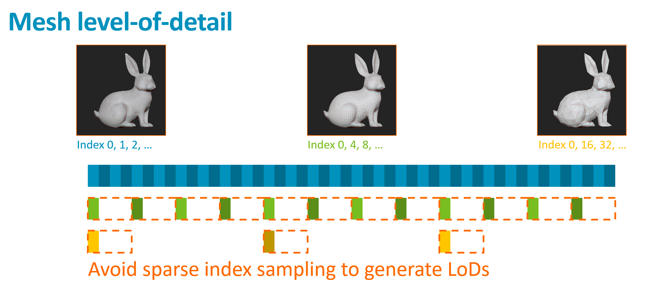
❌ 错误做法:共享顶点缓冲,通过索引跳取
蓝色兔子:使用全部顶点
绿色兔子:每 4 个顶点取 1 个
黄色兔子:每 16 个顶点取 1 个
问题:绿色兔子着色量 = 蓝色兔子(同一 4 顶点块被触发)
      → 简化网格零收益!
正确做法:独立顶点缓冲
| 策略 | 内存 | 带宽 | 着色量 |
|---|---|---|---|
| 每 LOD 独立缓冲 | 增加 | 仅加载所需 LOD | 最小 ✅ |
| 共享缓冲跳取索引 | 节省 | 可能相同 | 无优化 ❌ |
💡 游戏行业通常做对了这一点
三角形 vs 法线贴图
核心原则
不要用三角形建模一切 —— 尤其对 Tile-Based 渲染器
| 方法 | 优势 |
|---|---|
| 法线贴图 | 可纹理过滤、可压缩、低带宽、视觉效果更好 |
| 高模几何 | 仅在轮廓需要真实位移时必要 |
常见问题领域
- ❌ 汽车仪表盘 / 车载娱乐系统
- ❌ 嵌入式应用(非游戏背景开发者)
- 过度使用几何建模而非纹理
索引驱动顶点着色:内存布局优化
回顾:两阶段着色管线
Position Shading → 剔除/Tiling → Varying Shading(仅可见顶点)
缓存行问题
Mali 缓存行大小:64 字节
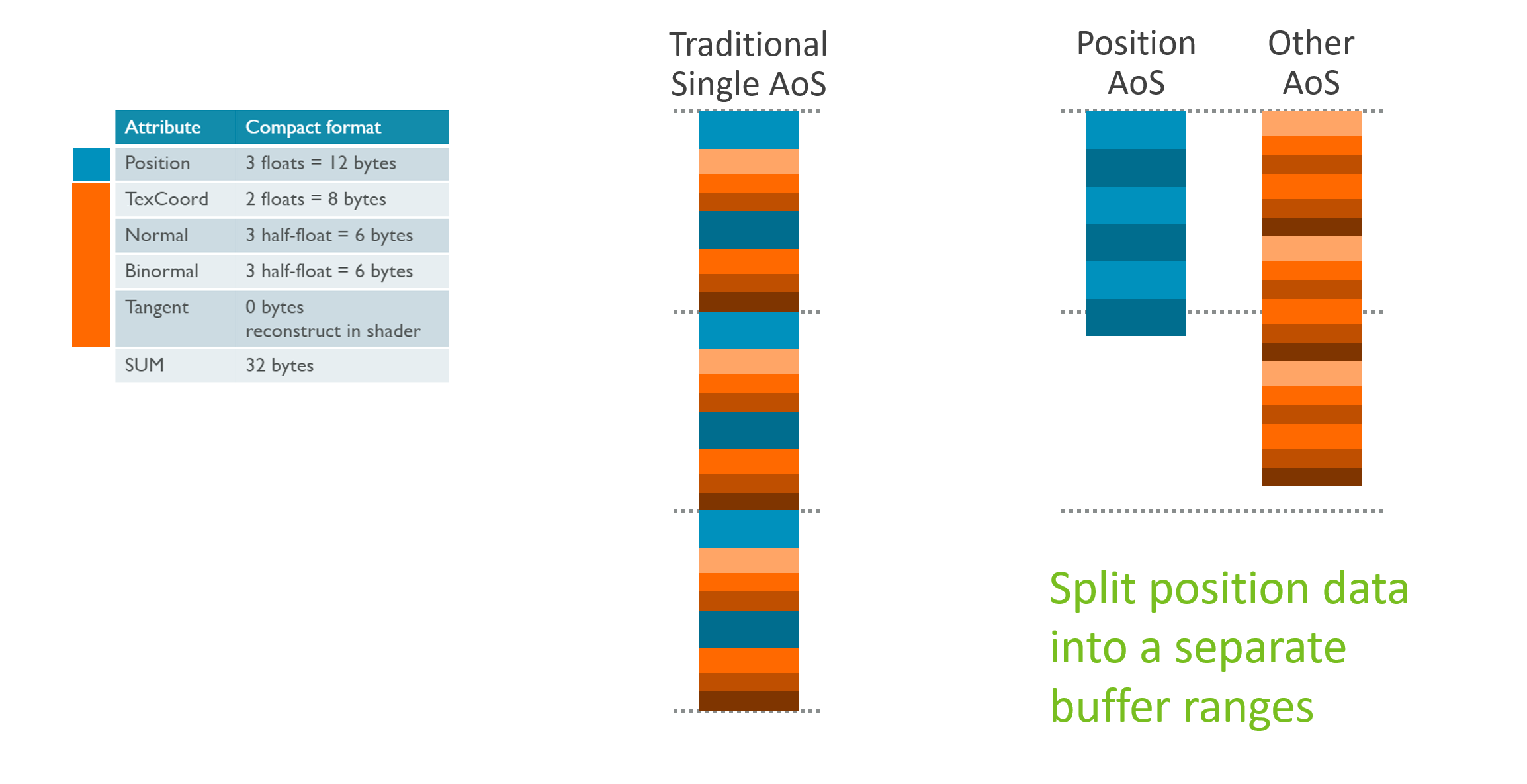
❌ Array of Structures(交错布局)

Position Shading 加载:24B 有用 + 40B 无用
带宽浪费:62.5%
正确做法:分离缓冲区
✅ Structure of Arrays(分离布局)

Buffer A: [Pos|Pos|Pos|Pos|...]    ← Position Shading
Buffer B: [UV|Normal|UV|Normal|...] ← 仅可见顶点加载

优势:
• 100% 有用数据
• 更少缓存行 → 更低延迟
• 最大化 IDVS 带宽节省
2D/UI 几何优化
全屏四边形的隐藏成本
两三角形全屏 Quad
对角线上的像素被着色两次
(2×2 Quad 规则)
1080p 约 0.5% 过度着色
解决方案:超大单三角形 + Scissor
使用 4K×4K 单三角形覆盖 1080p 区域
Scissor 裁剪到屏幕 → 无接缝 → 零过度着色
圆角 UI 的灾难模式
❌ 三角形扇形(Triangle Fan)
 • 大量细长三角形
 • 光栅化器高负载
 • 4× 过度着色
 • Tile 列表膨胀
正确做法:递归最大面积三角化
✅ 递归细分算法
1. 从最大三角形开始
2. 递归细分改善圆弧精度
3. 最小化边数
性能提升:3-5× (圆形表盘等场景)
⚠️ 避免细长对角三角形 —— 对光栅化 GPU 极不友好
纹理优化基础
核心原则
| 原则 | 说明 |
|---|---|
| 合适分辨率 | 避免过大纹理 |
| 正确颜色格式 | 匹配实际需求 |
| 使用压缩 | ETC / ETC2 / ASTC |
| 3D 内容必用 Mipmap | 提升缓存效率 + 视觉质量 |
过时技术警示
❌ ETC1 双采样 Alpha 技巧(已过时)

旧做法:图像宽度翻倍
左半:RGB    右半:Alpha(灰度)
需两次采样恢复 RGBA

✅ 现代方案:ETC2 原生 RGBA 压缩
纹理压缩、过滤成本与 Overdraw 优化
ASTC 纹理压缩格式
格式优势
| 特性 | 说明 |
|---|---|
| 发明者 | ARM(Mali 团队) |
| 标准化 | 2D LDR 在 OpenGL ES 3.2 强制支持 |
| 质量 | 比 ETC2 高约 0.25-0.5 dB(即使码率低 10%) |
| 灵活性 | 多种码率与颜色格式可选 |
HDR 支持现状
| 厂商 | 2D HDR Profile |
|---|---|
| Mali | ✅ |
| Adreno | ✅ |
| 部分其他厂商 | ❌ |
官方压缩工具:astcenc
- GitHub 开源
- 专用法线贴图/遮罩贴图误差模式 → 高质量法线压缩
- 性能优秀
Decode Mode 扩展
VK_EXT_astc_decode_mode / GL_EXT_texture_compression
作用:降低解压后中间精度
收益:命中 Mali G77+ / Valhall 快速纹理路径
✅ 推荐:尽可能启用
纹理过滤成本详解
过滤模式对比
| 模式 | 周期 | 带宽 | 视觉效果 |
|---|---|---|---|
| Bilinear | 1 | 1x | 基准 ✅ |
| Trilinear | 2 | 最高 5x | 消除 MIP 边界 |
| Aniso 2x + Bilinear | 1-2 | 中等 | 斜面清晰 |
| Aniso 2x + Trilinear | 1-4 | 较高 | 更平滑 |
| Aniso 4x + Trilinear | 最高 8 | 最高 64x | 最佳但昂贵 |
各向异性过滤原理
Anisotropic Filtering 工作方式

• 对每个像素做基于 patch 的积分
• 从高细节 MIP Level 采样多次
实用建议
| 场景 | 推荐 |
|---|---|
| 默认选择 | Bilinear(1 周期) |
| 需要平滑 MIP 过渡 | Trilinear(固定 2 周期) |
| 斜面纹理 | Aniso 2x + Bilinear(可能 ≤ Trilinear) |
| 高质量需求 | Aniso 2x + Trilinear(值得尝试) |
| 4x+ 模式 | 谨慎使用 |
💡 Max Anisotropy 不必是 2 的幂 —— 可用 2、3、4、5 等
相机/YUV 纹理
❌ 自行映射并软件转换颜色空间
✅ 使用扩展直接访问 YUV 数据
   • 硬件自动处理多平面表面
   • 硬件自动处理颜色空间转换
Overdraw 优化
问题场景
典型案例:视差滚动背景(Parallax Sidescroller)
7 层视差背景

Layer 7 ████████████████████████
Layer 6 ██████████████████████████
Layer 5 ████████████████████████████
...
Layer 1 ██████████████████████████████████

中部重叠区域:6x Overdraw!
预算冲击
| 目标设备 | 可用周期/像素 | 6x Overdraw 影响 |
|---|---|---|
| 低端机 1080p@60 | 6-10 周期 | 预算耗尽 |
⚠️ 这还只是背景 —— 游戏元素、特效还没算!
常规做法 vs 优化做法
❌ 常规做法:
• 裁切想要的形状
• 整体开启混合渲染
• 所有像素都经过片段着色
✅ 优化做法:分离不透明与透明
每层分割为两部分:
1. 找出完全不透明区域
2. 用最少额外顶点裁切出来
3. 作为 Opaque Draw Call 绘制(禁用混合)
4. 裁切剩余透明部分
5. 作为 Transparent Draw Call 绘制

收益:
• 不透明部分参与 Early-ZS / HSR
• 显著减少实际着色像素数
遗留技术警示
⚠️ 警惕"因为一直这么用"而保留的旧技术
许多场景现在有更好的替代方案,特别是配合 ASTC 等现代格式
2D 渲染优化与着色器编程技巧
2D 渲染中的 Overdraw 优化
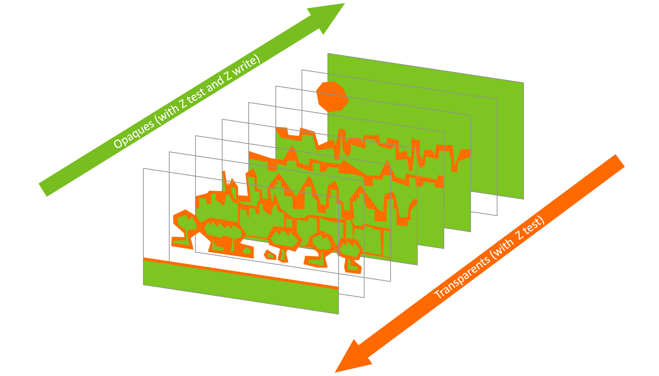
绘制分类
| 类型 | 示例颜色 | 特性 |
|---|---|---|
| 不透明(Opaque) | 🟢 绿色 | 完全遮挡后方 |
| 透明(Transparent) | 🟠 橙色 | 需要正确混合 |
理想绘制顺序
最佳方案:
1. 为每层分配 Z 值
2. 不透明:前到后 → 最大化 Early-ZS
3. 透明:后到前 → 正确混合
现实妥协方案
| 方案 | 实现难度 | 效果 |
|---|---|---|
| 全部后到前(按层) | 易于改造现有 2D 引擎 | 次优但可接受 |
| 理想排序 | 需要重构 | 最优 |
收益:
- 起始:峰值 5x Overdraw
- 优化后:平均 <2x Overdraw
- 来源:Early-ZS 或 HSR 的共同作用
着色器精度选择
mediump(FP16)的优势
| 指标 | 相比 highp(FP32) |
|---|---|
| 能耗 | 减半(翻转一半晶体管) |
| 寄存器占用 | 减半 |
| 吞吐量 | 2倍(vec2 → vec4 路径) |
必须使用 highp 的场景
| 场景 | 原因 |
|---|---|
| 位置计算 | 精度要求高 |
| 深度计算 | 避免 Z-fighting |
| 纹理坐标计算 | 避免采样偏移 |
精度转换成本
⚠️ mediump ↔ highp 转换不是免费的!
需要额外指令进行格式转换
→ 若只为省 1 条 highp 指令而转换,得不偿失
浮点数学的编译器限制
为什么编译器不自动优化?
示例代码:
// 原始
result = tex1 * scale + tex2 * scale;

// 数学上等价
result = (tex1 + tex2) * scale;  // 少一次乘法
问题:浮点数学 ≠ 实数数学
溢出示例
// FP16: max = 65504
float A = 65504.0;
float B = 65504.0;
float scale = 0.5;

// 原始:(A * 0.5) + (B * 0.5) = 32752 + 32752 = 65504 ✅
// "优化":(A + B) * 0.5 = ∞ * 0.5 = ∞ ❌
💡 编译器必须保守,因为无法假设不会溢出
整数 vs 浮点优化自由度
| 类型 | 编译器优化空间 |
|---|---|
| 整数 | 较大 |
| 浮点 | 受限(溢出、NaN、精度损失) |
内置函数使用指南
推荐使用内置函数
示例:颜色键检测
// ❌ 手写:5 条指令(Mali T860)
if (color.r == key.r && color.g == key.g && color.b == key.b) ...

// ✅ 内置:3 条指令
if (all(equal(color.rgb, key.rgb))) ...
优势:
- 更可读
- 有硬件支持或手写汇编优化
高成本内置函数
| 函数类别 | 示例 | 注意 |
|---|---|---|
| 三角函数 | sin, cos, tan | 不是免费的 |
| 双曲函数 | sinh, cosh, tanh | 同上 |
| 反三角函数 | asin, acos, atan | 同上 |
| 原子操作 | atomicAdd 等 | 大多数 GPU 上较慢 |
| 手动梯度采样 | textureGrad | 当前硬件昂贵 |
Uniform 计算优化
问题识别
// 仅依赖 uniform 的计算 → 每个线程结果相同
vec3 lightDir = normalize(u_lightPos - u_cameraPos);
驱动优化的局限
- 驱动 可以 优化但需要额外周期检测
- 最佳做法: CPU 预计算,上传修改后的 uniform
着色器特化策略
-
控制流特化:将
if/else分支直接编译成不同版本的 Shader,避免 GPU 在运行时重复执行逻辑判断。 -
循环限制常数化:将循环次数从变量(Uniform)改为常数(Literal),让编译器能实现循环展开(Unrolling)。
-
数据常量化:把固定不变的参数直接写死在代码里(常量),让编译器能进行表达式预计算和指令压缩。
-
避免无效实例化:在只画一个物体时,不要使用实例化绘图(Instanced Drawing),因为通过索引(如
gl_InstanceID)访问数据比直接访问普通 Uniform 慢。
问题:通用着色器
// ❌ 过于通用
if (u_mode == 1) { ... }
else if (u_mode == 2) { ... }
else if (u_mode == 3) { ... }
解决方案:编译时特化
// ✅ 使用宏特化
#ifdef MODE_1
    // 直接执行模式 1 逻辑
#endif
权衡
| 因素 | 特化程度高 | 特化程度低 |
|---|---|---|
| 运行时性能 | ✅ 更好 | ❌ 分支开销 |
| 着色器变体数 | ❌ 增多 | ✅ 更少 |
| 批处理能力 | ❌ 更难 | ✅ 更容易 |
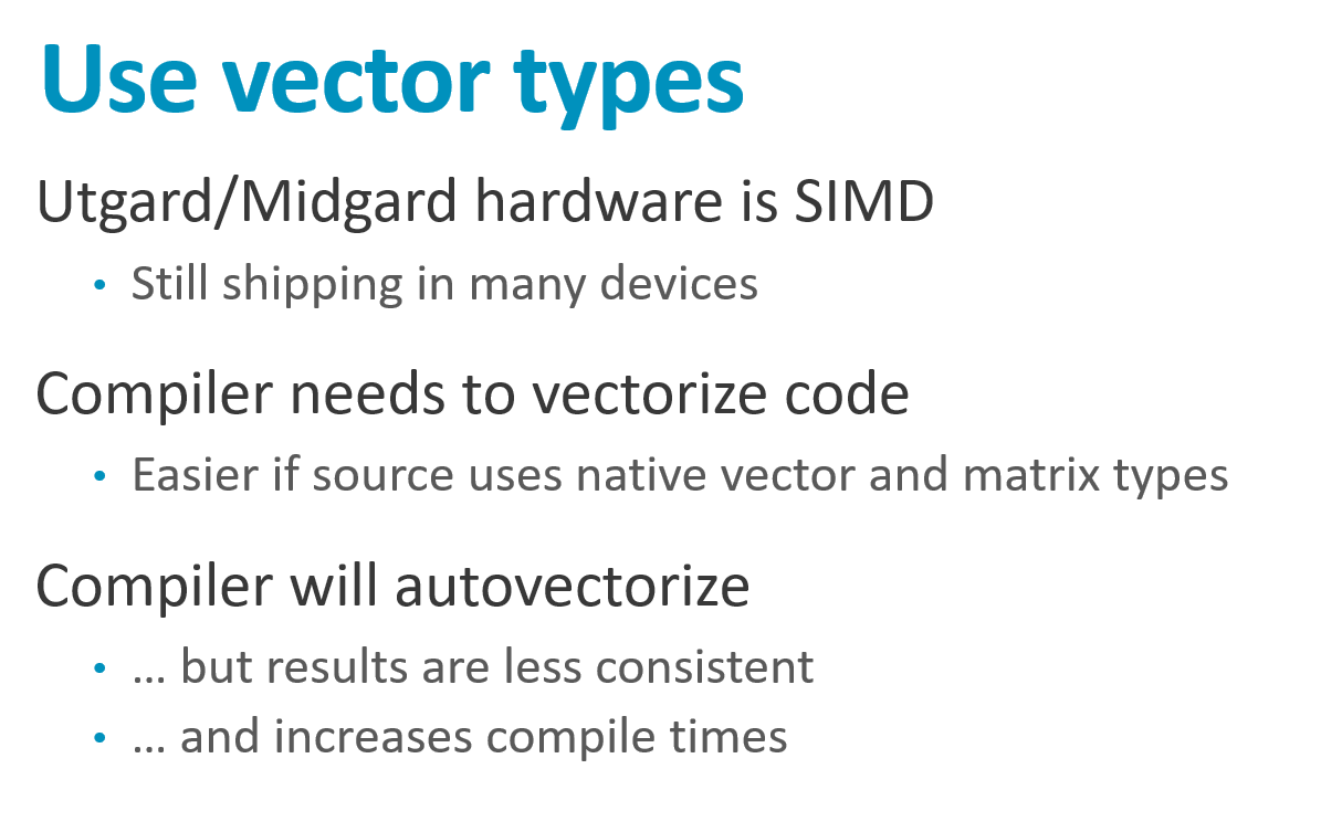
向量类型与 GPU 架构演进
不同架构建议
| 架构 | 特性 | 向量类型建议 |
|---|---|---|
| Midgard | SIMD | ✅ 使用 vec/mat 帮助向量化 |
| Bifrost/Valhall | 标量 | 影响较小 |
GPU 分支的演进史
GPU 分支能力演进
早期 GPU → 无分支 → 全展开 → 极其昂贵
SIMD GPU → 有分支 → 分歧时所有路径都执行
现代 GPU → 分支更便宜 → 但仍非免费
⚠️ 网上很多分支相关信息已过时 —— 请以当前硬件特性为准
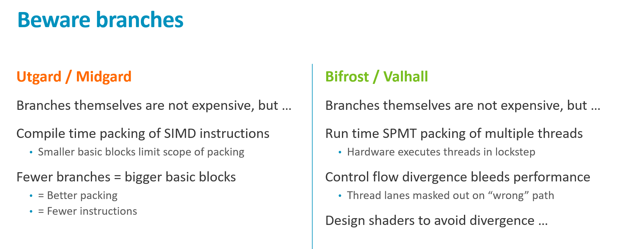
分支、Compute Shader 与优化优先级总结
分支指令的代际差异
旧架构(Midgard)的分支代价
| 问题 | 说明 |
|---|---|
| 分支本身 | 便宜 |
| 真正代价 | 编译器无法跨分支边界重排打包 SIMD 指令 |
新架构(Bifrost+)的分支特性
| 特性 | 说明 |
|---|---|
| Warp 执行模型 | 分支便宜,无打包问题 |
| 唯一关注点 | 控制流发散(Divergence) |
8 线程 Warp:4 走 if,4 走 else
→ if 分支:50% 占用率(4 线程被 mask)
→ else 分支:50% 占用率
→ 性能侵蚀!
Midgard 分支优化实例:光照计算
"聪明"的分支版本
// 尝试跳过远处光源
for (each light) {
    if (distance < cutoff) {
        do_light_calculation();  // 只算近处光
    }
}| 路径 | 周期 |
|---|---|
| 最短(无光可见) | 5 |
| 最长(3 光全算) | 13 |
移除分支后
// 始终计算所有光源
for (each light) {
    do_light_calculation();
}| 路径 | 周期 | 变化 |
|---|---|---|
| 最短 | 7 | +2 |
| 最长 | 7 | -6(近半!) |
💡 Midgard 经验: 计算往往比避免计算更便宜
分支处理建议总结
| 架构 | 建议 |
|---|---|
| Midgard | 谨慎使用分支,优先无分支计算 |
| Bifrost+ | 分支基本免费,别过度优化 |
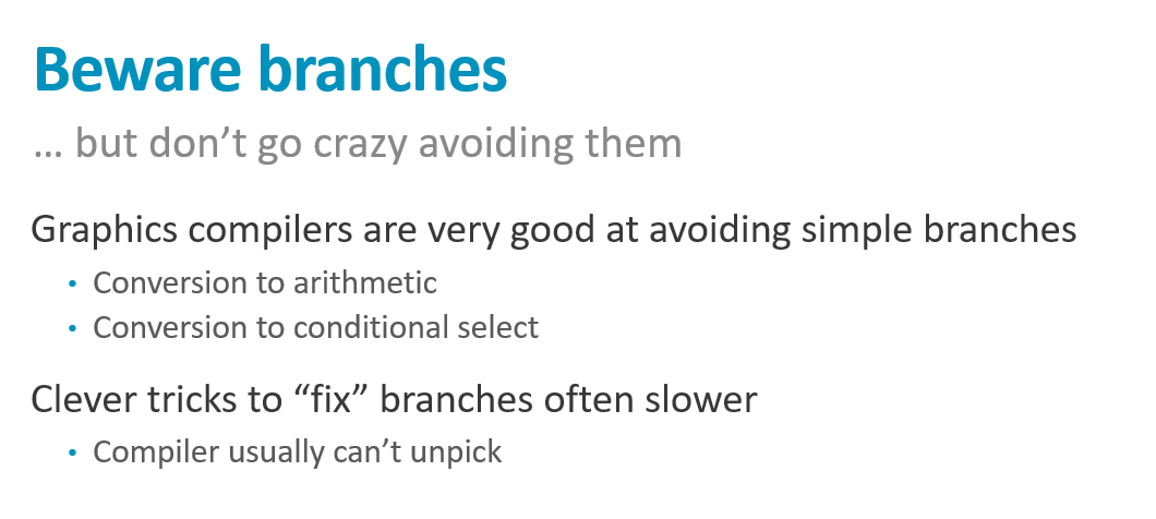
⚠️ 别用复杂数学替代简单 if —— 编译器会自动插入 conditional select / MOV
向量打包与属性布局
加载效率
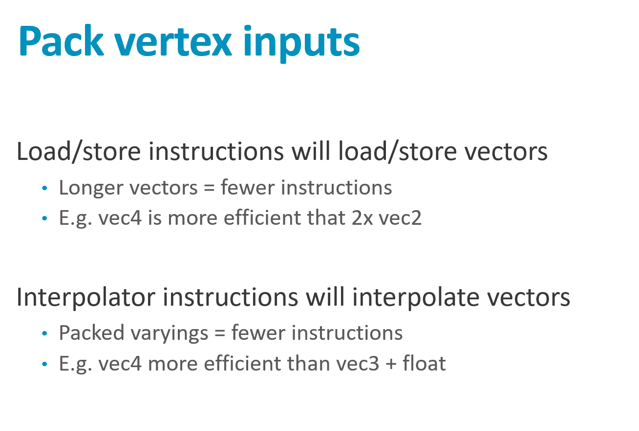
| 方式 | 效率 |
|---|---|
vec4 | ✅ 最佳 |
2 × vec2 | 次优 |
vec3 + float | ❌ 浪费 |
建议: 打包属性、最小化 padding
Late ZS 触发条件
触发 Late ZS 的操作
| 操作 | 后果 |
|---|---|
discard | Late ZS 更新 |
修改 gl_FragDepth | Late ZS + 禁用 HSR |
| 读取帧缓冲 | 等效透明 → Late ZS + 禁用 HSR |
使用建议
- 合理用途(如树叶 Alpha Test)→ 正常使用
- 不需要时 → 禁用
- 确保安全时 → 使用
layout(early_fragment_tests) in;强制 Early ZS
Compute Shader 优化
Work Group 大小
| 推荐 | 说明 |
|---|---|
| 64 work items | 良好起点 |
| Warp 倍数 | 避免部分填充 |
| 尺寸 | 问题 |
|---|---|
| 过大 | Barrier Resolve耗时长 |
| 过小 | 无法填满 Warp,算法效率低 |
💡 最优值因 GPU/厂商而异 → 可在安装时测试
Mali Local Memory(Workgroup Shared Memory) 陷阱
Mali:Local Memory = Load/Store Cache 支持
      无专用硬件 RAM!

❌ 桌面 GPU 技巧:Global → Local 作为加速池
   Mali 上反而污染缓存,性能下降

✅ 正确用法:仅用于算法需要的线程间共享
优化总结:Top 6 优先级
核心原则
| 优先级 | 说明 |
|---|---|
| 少做 > 快做 | 减少工作量 > 优化执行速度 |
| 提前预算 | 尤其针对大众市场设备 |
六大优化焦点
| # | 领域 | 关键点 |
|---|---|---|
| 1 | Frame Graph | 数据流干净 → 保住 Tile-Based 优势 |
| 2 | Mesh LOD | 远处简化网格 |
| 3 | 三角形打包 | 属性精度、索引驱动顶点着色兼容 |
| 4 | 着色器精度 | mediump 优先 → 省电/省寄存器/省带宽 |
| 5 | Specialization | 特化变体 |
| 6 | Overdraw | UI 层叠尤其严重(可达十几层) |
💡 十年经验: 问题通常出在这 Top 6,很少需要更深入优化