Graphics101

Arm GPU Training Series Ep 1.1 : Introduction to mobile systems

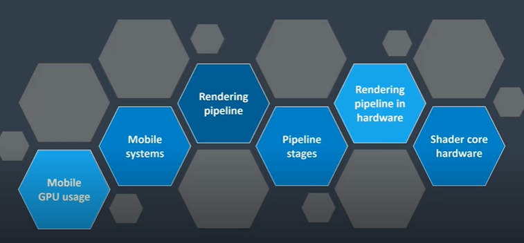
Overview of Training Modules

Over the next few days, we will be covering three training modules. The first module will focus on general mobile best practices. This module is not specifically related to Mali, but it establishes the baseline problem that mobile optimization is trying to solve. We will cover this module this morning (or this evening, depending on your time zone).

Tomorrow's module will dive into Mali best practices, focusing specifically on the Mali GPU. We'll discuss recommended development methodologies and other practices that we advise for optimizing performance.

The final module on Wednesday will explore Mobile Studio in greater detail, including the features of the tools for pro and what you can achieve with them. Much of the content in this module is also applicable to Development Studio, as many of the tools are shared between the two. For example, the Streamline part is common to both.

Interaction and Clarifications

I am happy to answer any questions as we progress through the modules. If anything is unclear or if I am moving too quickly, please let me know. I tend to speak fast, even for native English speakers, so don’t hesitate to ask me to slow down if needed.

Today's Module: General Mobile GPU Usage

In this morning's module, we will quickly overview general mobile GPU usage. We will cover:

1. What Mobile GPUs are Used For

   We'll begin by discussing the primary uses of mobile GPUs and what this means within a mobile system.

2. Rendering Pipeline Overview

   We'll run through the rendering pipeline, which will be familiar if you've covered graphics before. This overview is essential as it highlights a few key points that will be crucial for tomorrow's module.

3. Real Hardware Implementations

   We'll discuss how these concepts translate into real hardware, focusing on Mali's tile-based rendering. We'll explore what this means and its implications for content efficiency.

4. Building Shader Cores

   Finally, we will examine the architecture of shader cores, discussing terms like warps and warp architecture. We'll explain what these mean and their implications for writing efficient graphic shaders.

Tomorrow's Module: Mali Best Practices

Tomorrow, we will revisit some of today's content from a Mali-specific perspective. We'll highlight key points and explain what they mean in terms of content behavior, providing a deeper understanding of how to optimize for the Mali GPU.

First Topic: Mobile GPU Usage

Let's begin by discussing mobile GPU usage.

Perceptions and Uses of Mobile GPUs

When most people think of mobile GPUs, they often associate them with 3D gaming. This is rooted in the heritage of desktop PCs and gaming consoles, and it is indeed a growing market in mobile devices. Popular titles like Fortnite, PUBG, and Honor of Kings are prime examples of 3D games deliberately targeting mobile platforms with high-end graphics.

However, the majority of mobile game titles are actually 2D. Today, approximately 75% of game titles on the Google Play Store are 2D games. These games are designed to run on a wide range of devices, from entry-level phones to the latest high-end models. Despite their simpler graphics, these 2D games can still face performance issues, particularly on lower-end devices.

GPU Usage Beyond Gaming

Beyond gaming, nearly all mobile platforms use the GPU to render the entire operating system's user interface (UI). While some software rendering may be used initially to generate tiles or texture data, the final composition is handled by the GPU. For example, on Android devices, the home screen is a native 3D application, with elements like live wallpapers being rendered in real-time by the OS compositor. This makes energy efficiency critical for mobile GPUs, as they are constantly engaged in rendering both the OS-level UI and the graphics behind web browsers and other applications.

Integration with Video Sources

Mobile GPUs are also designed to integrate with a wide variety of video sources. This includes set-top boxes that consume cable or satellite streams, as well as smartphones handling camera inputs or video playback. It is crucial for the GPU to efficiently process video streams and camera images, not just the traditional RGB color data used in graphics. To support this, mobile GPUs can directly access YUV-encoded data in addition to the usual RGB data provided through APIs.

Expanding Roles of GPUs

Increasingly, GPUs are being used for more than just traditional graphics tasks. The GPU is an excellent data-domain parallel processor, which is why it excels in graphics—a highly data-parallel problem. However, this architecture also generalizes well to other data-parallel problems, such as computer vision, where parallel algorithms process images or sensor data to infer object classification or meaning.

Moreover, GPUs are increasingly utilized in machine learning, particularly for running neural networks. This involves large matrix multiplications, a type of workload that GPUs handle exceptionally well. As a result, the role of the GPU is expanding beyond graphics into other domains that benefit from parallel processing capabilities.

Optimizing Workloads on Mali and Mobile Systems

We are focusing on optimizing various workloads on Mali, particularly in the context of mobile and Android systems. This brings us to the topic of mobile systems and the considerations for targeting content on such platforms. One key aspect to consider is the performance budget available in mobile systems, such as Samsung devices.

The Main Rendering Pipeline

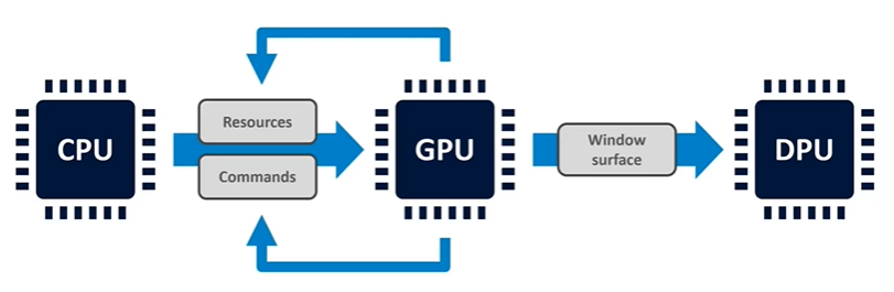
The main rendering pipeline in a mobile system involves several key components. First, the CPU runs the application and the graphics driver, which in turn feeds the GPU. The GPU consumes resources such as textures, shader programs, and data, along with a set of commands that instruct it to process these resources. These commands typically come from the graphics API and may include tasks like draw calls or compute dispatches. At the end of a frame, the GPU produces a completed window surface, which is then handed off to the display processor.

Differences Between Desktop and Mobile Graphics Systems

In traditional desktop graphics systems, such as those in PCs, the display processor is typically integrated into the GPU. However, in mobile systems, the display processor is often a separate piece of IP (intellectual property), sometimes developed by a different company. When we refer to the Mali GPU, we are specifically talking about the part of the system that handles rendering. It writes the completed frames back to main memory, while a different block of IP handles the display output.

Advanced Capabilities of Modern GPUs

Modern GPUs have advanced capabilities that go beyond basic rendering. For example, GPUs can now generate their own resources and modify their own command streams. This enables more complex rendering pipelines with effects generated by the GPU itself. Techniques like rendering back into a texture allow for intricate visual effects, all managed internally by the GPU.

Furthermore, features like draw indirect and multi-draw indirect allow the GPU to modify the tasks assigned by the CPU. While current APIs do not yet support fully general-purpose command generation by the GPU, the trend is moving towards increased self-command submission. This shift enables the CPU to offload more work to the GPU, ultimately reducing the CPU load and improving overall system performance.

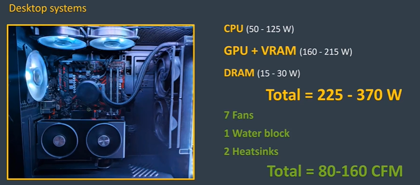
Graphics Optimization in Gaming PCs vs. Mobile Devices

When people think of graphics optimization, they often start with a traditional gaming PC. In a mid-range gaming system with standard components (nothing overclocked), power consumption typically falls between 200 and 400 watts for the CPU, GPU, and DRAM combined. This high power consumption is sustainable because gaming PCs are equipped with extensive cooling systems, including large heatsinks, water blocks with radiators for the CPU, and multiple fans. Every watt of energy consumed translates to waste heat that must be to maintain performance. The cooling systems allow a high power budget, with airflow ranging between 80 and 160 cubic feet per minute.

Mobile System Architecture

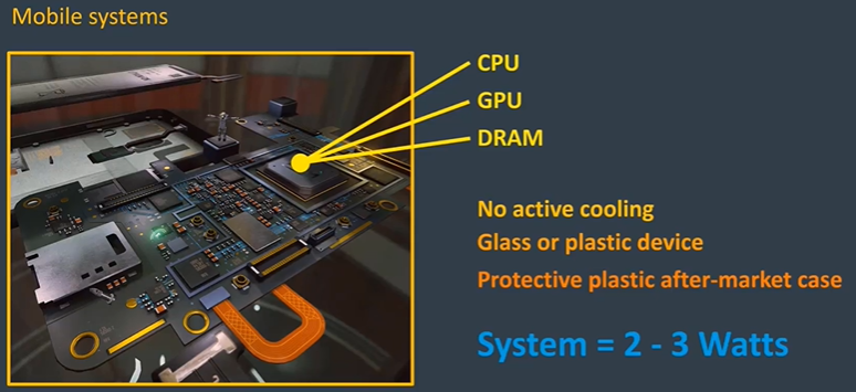
In contrast, mobile systems are much smaller and typically use a single system-on-a-chip (SoC) architecture. These SoCs often consist of two or three logic dies stacked on top of each other, containing the main logic (CPU, GPU, and accelerators) and DRAM. This package-on-package arrangement is efficient, simplifying the circuit board by reducing the number of wires. However, it also means that all major heat-generating components are concentrated in one area, making heat dissipation a challenge.

Moreover, mobile devices lack active cooling systems—there are no fans or heatsinks. These devices are usually made of insulating materials like glass or plastic, and users often add aftermarket cases, further insulating the device. This situation imposes a very strict thermal budget on mobile gaming, with the entire system (excluding the display) typically limited to a thermal budget of just 2 to 3 watts. This is a mere 1% of what a desktop PC might use, making power management crucial.

The Strict Power Budget of Mobile Devices

To put this into perspective, even the most energy-efficient LED bulbs, which are equivalent to 40-watt incandescent bulbs, consume about 5 watts. In comparison, mobile devices must operate on an even stricter power budget. Despite these limitations, mobile devices still manage to perform complex tasks, albeit within these tight constraints.

CPU Architecture in Mobile Systems

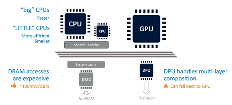
The main rendering subsystem inside most mobile SoCs features multiple types of CPUs. These include "big" CPUs, which are physically larger and significantly faster, offering the highest single-thread performance. Alongside these, there are "little" CPUs—smaller, more energy-efficient cores with lower peak single-thread performance. Some designs also include "medium" CPUs, creating a mix of 2 bigs, 2 mediums, and 4 littles, or variations thereof.

The operating system dynamically balances workloads across these CPUs based on demand. Light workloads run on medium or little CPUs, while heavy single-thread workloads are assigned to the big CPUs for maximum performance. All these CPUs share some level of L3 cache, ensuring coherence across the system. Additionally, there may be a system cache between the IP and DRAM, depending on the silicon partner involved.

The Role of the GPU and Display Processor

The GPU in mobile systems plays a significant role in rendering and will be discussed in detail. Another crucial component is the display processor, which has evolved from being a simple controller to a sophisticated processing engine. It can perform various image processing tasks, such as rotation, scaling, and multi-layer composition. For example, in Android, the display processor might natively composite the home screen icons on top of the background. However, the display processor has its limits due to the real-time constraints of updating the display. If the workload becomes too complex (e.g., too many layers or high-resolution content), the system may offload these tasks to the GPU, which can quickly deplete the power budget.

Power Efficiency in Mobile CPUs

One of the most important considerations in mobile systems is power efficiency, especially when it comes to DRAM access, which is particularly power-hungry. As a rough estimate, memory traffic consumes about 100 milliwatts per gigabyte per second. Given the limited power budget (2-3 watts), even modest memory traffic can consume a significant portion of the available power, leaving little room for the CPU and GPU.

This power constraint is why mobile devices feature multiple CPU cores. Multithreading allows the system to spread workloads across several cores, enabling them to run at lower frequencies and, thus, higher energy efficiency. By running at lower frequencies, the CPU can significantly improve its performance-per-watt ratio, a crucial factor in maintaining overall system efficiency.

Conclusion

In conclusion, graphics optimization in mobile devices involves much more than just ensuring that shaders run efficiently. It requires careful consideration of the entire system's power and thermal constraints. Just as Peter Drucker emphasized in his management philosophy, effectiveness in optimization is about doing the right things, not just doing things right. This means selecting the right algorithms and balancing workloads to achieve the best possible performance within the strict power and thermal budgets of mobile devices.

The Cost of DRAM Access in Mobile Devices

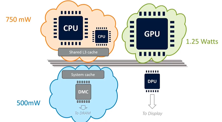
One of the most critical considerations for mobile devices is the energy cost associated with DRAM access. The process of communicating through the memory controller over the physical interface to the external DRAM is power-intensive. As a rough approximation, this process consumes about 100 milliwatts per gigabyte per second of memory traffic. This estimate can vary by about 30% depending on factors like process technology and DRAM technology. Given that most mobile devices operate within a strict power budget of 2 to 3 watts, DRAM access quickly becomes a significant factor. For instance, 5 gigabytes per second of memory traffic could consume around half of the available power budget, leaving very little for other components like the CPU and GPU.

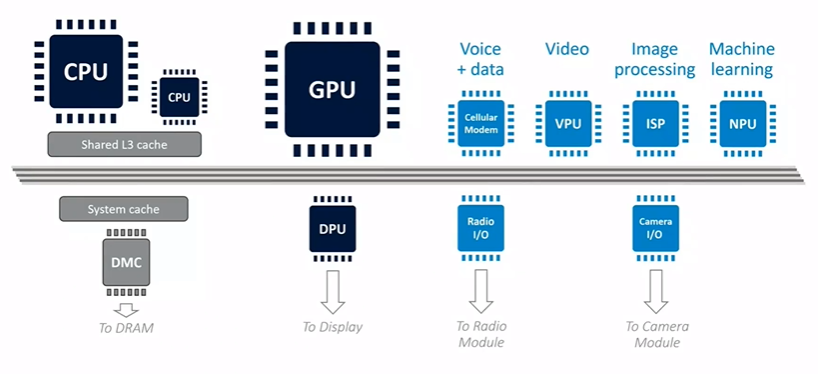
Domain-Specific Accelerators and Power Distribution

In addition to the main CPU and GPU subsystems, mobile devices include several domain-specific accelerators. These may include a modem for voice and data, video encode and decode units, an Image Signal Processor (ISP) for camera data, and specialized units for machine learning and location services like GPS. All these components share the same 2 to 3-watt power budget as the CPU and GPU. For example, a game like Pokémon Go, which uses the camera, data connection, and GPS, will have these components drawing power, reducing the available budget for rendering. This necessitates careful power management, as the entire system must operate within a very tight power envelope.

Understanding Power Efficiency in Mobile CPUs

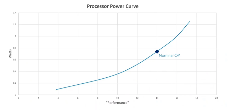
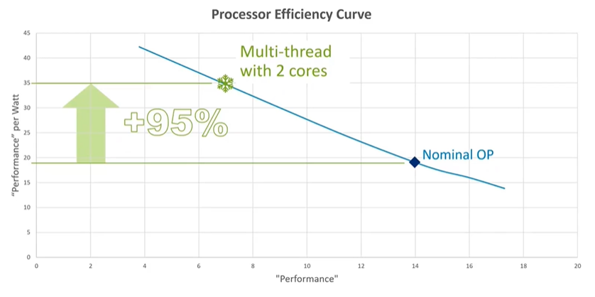
One of the most important graphs for understanding power efficiency in mobile devices is the performance-to-power consumption curve for a big Cortex CPU. Each silicon process has a nominal voltage, typically around 0.75 volts for modern processes. At this nominal voltage, a big Cortex CPU might consume around 750 milliwatts of power, delivering a certain level of performance. Overclocking the CPU increases performance but also steeply increases power consumption, making it less efficient. Conversely, underclocking the CPU reduces performance but significantly improves energy efficiency. For example, at its lowest frequency, a CPU might achieve 42 performance points per watt, whereas at its highest frequency, it might only achieve 13 performance points per watt. This trade-off highlights the importance of managing CPU frequency to optimize energy efficiency.

The Role of Multithreading in Energy Efficiency

Mobile systems often feature multiple CPU cores, not for sheer performance but for energy efficiency through multithreading. By running multiple threads in parallel across several cores, the system can operate at lower frequencies, which improves energy efficiency. Well-written software that supports multithreading allows these CPUs to run at lower, more energy-efficient operating points, thus extending battery life without sacrificing performance.

The Importance of Effectiveness in Optimization

Optimization in mobile devices isn't just about efficiency; it's about effectiveness. Peter Drucker, a renowned management consultant, once said, "Efficiency is doing things right; effectiveness is doing the right things." This philosophy applies to optimization as well. While it's important to have efficient code, it's even more crucial to ensure that you're using the right algorithms. An inefficient algorithm, no matter how well implemented, will always fall short compared to an effective one. Therefore, optimization should focus on choosing the right methods before worrying about the fine details of implementation.

Introduction to the Rendering Pipeline

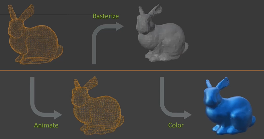
Next, let's quickly dive into the rendering pipeline, the core of the GPU. If you're already familiar with graphics, some of this might be a refresher. The process begins with a mesh, which represents the object as an infinitely thin skin—essentially hollow. The first step is to animate this mesh so that each vertex is positioned correctly on the screen for every frame. Afterward, the vertices are rasterized to determine which pixels need coloring. For each rasterized pixel, a fragment shader is applied to enhance its appearance. This, in essence, is the basic graphics pipeline. Although there are more stages, these are the fundamentals, especially for mobile graphics where many additional stages might not be used.

A Closer Look at the Rendering Pipeline

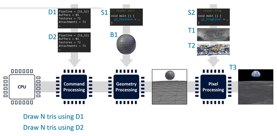
The rendering pipeline involves several key stages. While the CPU plays a role, our focus here is on the GPU's tasks. The command processing stage interprets instructions from the graphics driver, followed by geometry processing, where input mesh data is transformed into screen-space triangles. These triangles then proceed to pixel processing, where they are colored.

The process begins with the application uploading resources such as graphics shaders, buffers, and textures. Descriptors, essentially data structures, guide the GPU on where to find these resources and what parameters to use (e.g., blending, depth testing). The CPU then submits commands, like "draw triangles using descriptor set 1," which are read by the command processor and passed through the geometry and pixel processing stages. This process is repeated, often thousands of times per frame, to render the final image on the screen.

The Role of Compute in the Pipeline

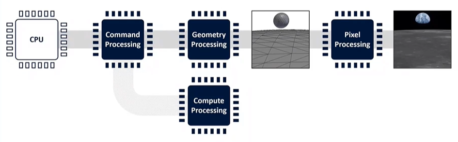
Compute operations, which use the GPU as a general-purpose processing engine, operate outside the main rendering pipeline. These operations can read inputs from and write outputs to main memory, interacting with other pipeline stages as needed. While not part of the fixed-function pipeline, compute is crucial for certain tasks, even though it's not discussed extensively here.

Geometry Processing: A Multi-Stage Pipeline

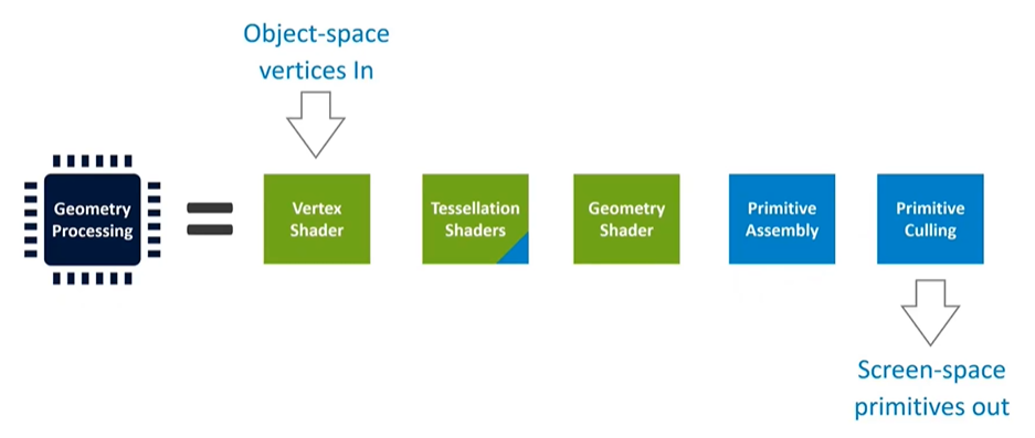
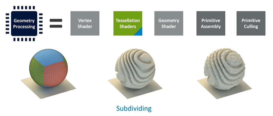
Geometry processing involves multiple stages. The green stages represent application programs, like shader programs provided by the application. The blue stages are fixed-function stages that can be configured but not fundamentally altered by the application. Tessellation, for instance, is a multi-stage process that starts with object-space vertices and outputs screen-space triangles ready for rasterization and pixel coloring.

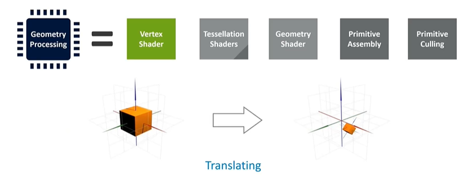
The vertex shader handles translations and computations for each vertex, taking them from object space to screen space. Tessellation, a powerful yet resource-intensive technique, can subdivide triangles to add detail. However, due to its complexity and high cost, tessellation is rarely used in mobile applications outside of benchmarks.

Procedural Geometry and the Inefficiencies of Geometry Shaders

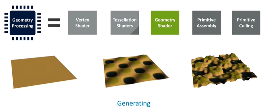
Geometry shaders were once popular for tasks like particle systems and explosions, but they are now considered inefficient on modern GPUs. These shaders force duplication of triangles, which is highly inefficient. Instead, compute shaders are recommended for such tasks. While geometry shaders are supported in APIs, they are rarely used in real-world mobile content.

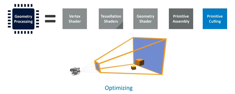
Fixed-Function Stages and Culling

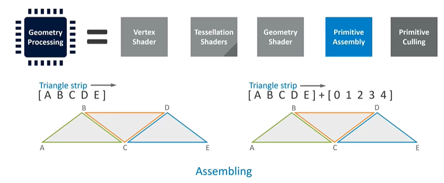
After geometry processing, the final fixed-function stages assemble the vertices back into triangles. These triangles undergo culling, where the system determines what's within the camera's frustum and discards anything outside it. Unfortunately, traditional pipeline designs place culling at the end, meaning a lot of work is done only to discard triangles later. This is inefficient, so many modern GPUs reorder the pipeline to perform culling earlier, reducing redundant work.

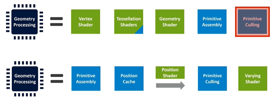
Optimizing the Pipeline for Efficiency

In the current generation of Mali GPUs, the vertex shader is split into two parts: one that computes position and another that handles additional vertex data. The second part only runs for triangles that survive the culling process, significantly improving efficiency. This approach ensures that only necessary work is done, with efficiency gains increasing if the application passes in data outside the camera's frustum. This optimization is common in modern hardware and helps minimize redundant work, enhancing overall performance.

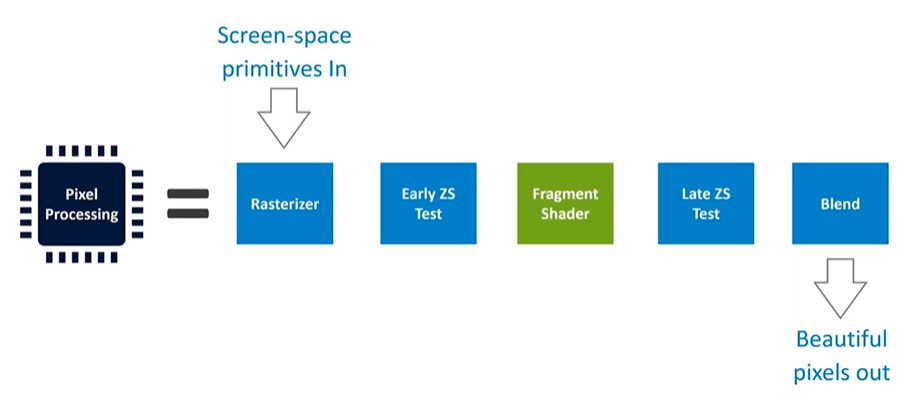
Pixel Processing Overview

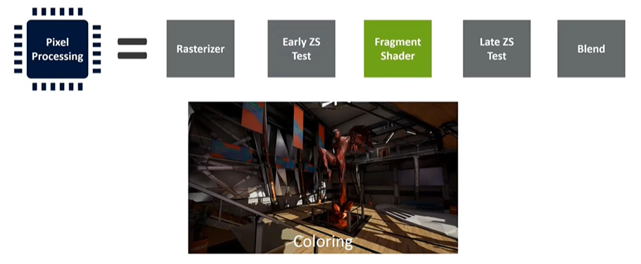
On the pixel processing side, there is a substantial amount of fixed-function hardware. This includes rasterization, two layers of depth testing (early and late), and the fragment shader, which runs the user program. There is also fixed-function logic for tasks like blending before outputting the final image to the frame buffer. The goal of this stage is to transform screen-space primitives from earlier stages into beautifully rendered pixels.

Rasterization Process

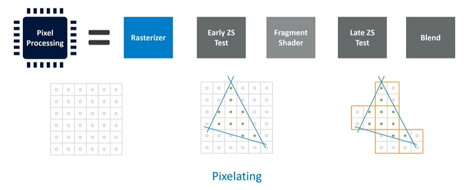
Rasterization takes the vector form of triangles generated by vertex shaders and tests them against discrete sample points per pixel. An important detail about rasterization is that triangles are not processed as single fragments but as two-by-two pixel patches, known as quads. This approach is necessary for calculating derivatives (dX/dY) required for mipmap selection. However, the hardware will always process pixel shading in these quads. If a triangle only partially covers these sample points, the resources for the entire two-by-two pixel patch are still utilized.

For example, a triangle covering 10 pixels might actually occupy 20 pixels worth of screen area due to these partial quads, making small triangles disproportionately expensive. They require more vertices to cover the screen area, but the data is spread over fewer fragments, leading to an efficiency loss as not all threads are performing useful work.

Depth Testing and Fragment Shading

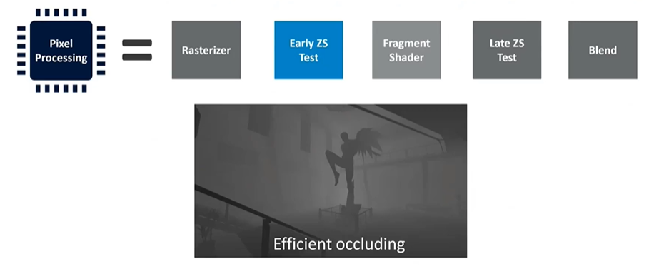
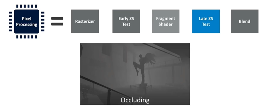
The early depth test occurs before shading, and if objects are rendered front to back, this test can cull objects hidden behind those already drawn. After fragment shading, another depth test—late depth test—takes place. This second test is for cases where the early test couldn’t be performed, such as when a fragment shader dynamically determines the depth value. In these scenarios, the shader program must run to completion before the depth value can be evaluated.

Blending and Pipeline Inefficiencies

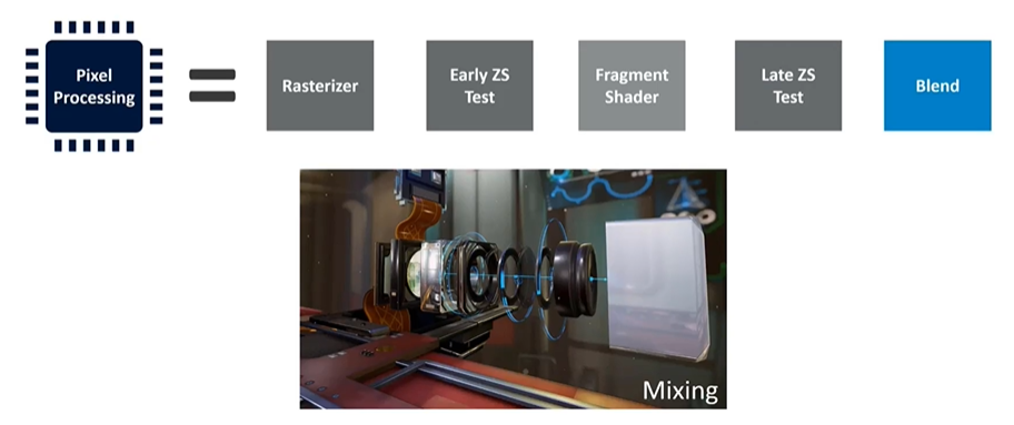
The final stage is blending, where transparent elements, like camera lenses, are merged with the background. However, this pipeline can be inefficient. For instance, the process requires the application to render in a front-to-back order for opaque objects to ensure the most conservative depth value is stored first in the frame buffer. If opaque layers are rendered back to front, they could fail the depth test because they appear closer than the previously rendered layer, leading to significant overdraw issues.

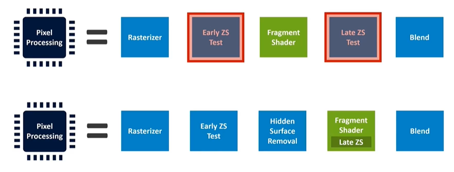
Similarly, while the late depth test happens after fragment shading in the specification, it is often possible to determine whether a pixel can be discarded early in the shader program. For example, with alpha-tested leaves, the shader first reads the alpha value to decide if the pixel should be discarded. This means the entire program doesn't need to run to determine if late depth testing can be resolved.

Optimizing the Pipeline for Efficiency

To address inefficiencies, modern GPU implementations often reorder the pipeline. One common addition is a hidden surface removal stage, which removes occluded elements that the early depth test cannot. Each GPU vendor has its proprietary method for this, though details are not publicly documented.

Another optimization involves moving late depth testing into the fragment shader, allowing the shader itself to trigger the test. This way, as soon as the shader has enough information, it can perform the depth test, and the remaining part of the shader program doesn't run if the pixel fails the test. This minimizes wasted computation. These optimizations are standard across modern GPUs, not specific to any particular architecture.

Introduction to Pipelining and Parallelism

When discussing pipelining in computing, it's helpful to think of a physical pipeline: as something is pushed in at one end, something must be dropping out at the other end because everything moves along inside the pipeline. This analogy is useful for understanding the concept of pipelines in computer science, where we aim to achieve continuous processing.

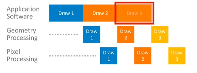
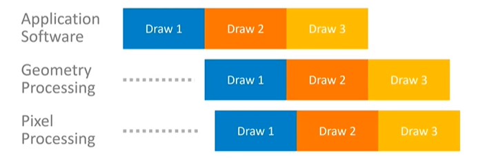
Concept of Pipelining in Graphics Processing

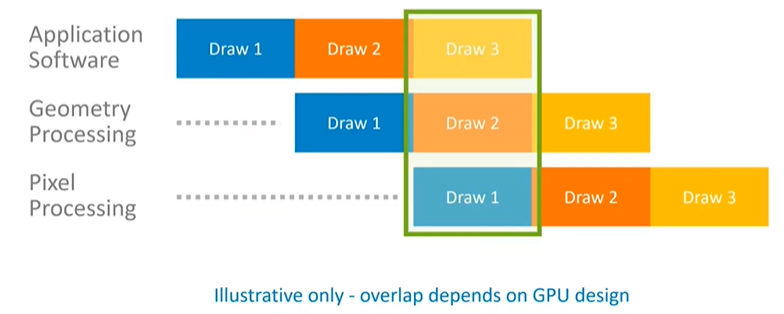
Conceptually, in graphics processing, the application builds a draw call and submits it to the geometry processing stage. Once geometry processing is complete, the draw call moves to pixel processing. The application doesn't need to wait for the result of each draw call because it knows that the result will eventually end up on the display. This allows the application to immediately start working on the next draw call and continue submitting them down the pipeline.

In a steady state, processing occurs in parallel across all pipeline stages, which keeps them busy and ensures the best performance. This parallelism allows the system to run at the lowest possible frequency, leading to greater energy efficiency. However, the degree of overlap and parallelism achievable depends heavily on the GPU design being used, so the general concept should be understood rather than assuming the specific diagram is universally representative.

Potential Pitfalls: Pipeline Draining and Serialization

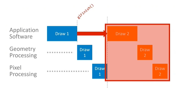
The application can disrupt this parallelism if it is not careful. For example, using the GL Finish API call in OpenGL ES drains the entire pipeline, blocking the CPU until all queued rendering is complete. This forces the geometry and pixel processing to run in sequence, meaning the CPU cannot start working on the next draw call until the current one has finished. This leads to serialized processing, where nothing happens in parallel, resulting in inefficient system use.

While GL Finish is a particularly bad example and not typically used in real applications, other API usage patterns can cause similar pipeline draining and serialization if not managed carefully. Ensuring the application avoids these drains is crucial, and best practices for API use will be covered in detail.

Identifying Bottlenecks in the Pipeline

Understanding where the critical parts of the pipeline are is essential for optimizing performance. In some cases, an application might be maxing out its performance, but not all processors are equally busy. For instance, if the application software is constantly busy but the GPU is idling between geometry processing and pixel processing tasks, the application is CPU-bound. Here, optimizing CPU behavior would be the key to improving performance.

In pipeline systems, the slowest stage typically determines overall performance, with other parts running in parallel but constrained by this bottleneck. Identifying this slow stage is crucial, and tools like Mobile Studio can assist in pinpointing and addressing these performance-limiting factors.

Introduction to GPU Architecture

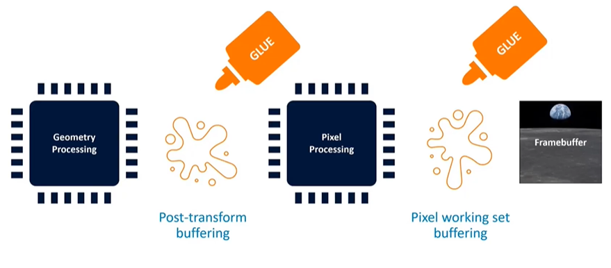
In this section, we'll explore GPU architecture to understand the context behind some of the best practices for optimizing performance, particularly in relation to Mali GPUs. We will focus on the two primary processing stages—geometry and pixel processing—and the various components that link them together. The way these components are organized can differ significantly between GPU vendors, which is a key area of differentiation in the market.

Key Processing Stages: Geometry and Pixel Processing

The GPU architecture consists of two main processing stages: geometry processing and pixel processing. These stages are connected by "glue" components, which manage the data flow between them. For example, there's typically a post-transform buffer that stores the output of the geometry processing stage before it is passed to the pixel processing stage. Additionally, the pixel processing stage outputs data that builds up in layers, such as depth testing, alpha transparency, and multi-sampling, contributing to a working set of the frame buffer.

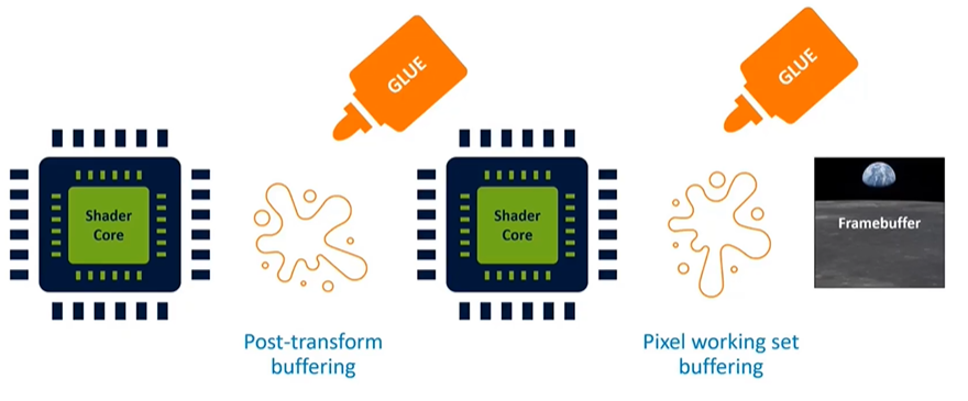
The Role of Shader Cores

Within these stages, shader cores play a critical role. These cores are specialized processors that run the shader programs responsible for rendering graphics. Unlike CPU cores, shader cores are optimized for the unique algorithms required in graphics processing, making them crucial to the performance and efficiency of the GPU.

Immediate Mode Rendering

To illustrate how these components work together, let’s consider an example using an immediate mode renderer. This is a traditional method, similar to what was used in early 3D graphics cards like the 3Dfx Voodoo. In immediate mode rendering, triangles are processed in the exact order that the application passes them to the GPU. For example, if you have a scene with a full-screen blue background and a green stripe overlaid on top, the GPU will render the blue triangles first, followed by the green ones.

Pipeline and Frame Buffer Interaction

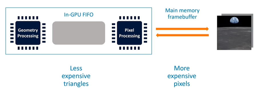
In an immediate mode renderer, the pipeline is structured as a First-In, First-Out (FIFO) queue. The output from geometry processing is stored in this small RAM buffer within the GPU and is then fed into the pixel processor. If the pixel processor is slower than the geometry processing, the FIFO buffer will eventually fill up, causing geometry processing to pause until there is space available in the buffer.

The frame buffer, which stores the final rendered image, is typically too large to fit entirely within the GPU. Therefore, it must be stored in the main memory. This leads to frequent round trips between the GPU and main memory to fetch and store frame buffer data, especially for operations like depth testing, blending, and multi-sampling. While techniques like frame buffer compression and caching can help mitigate the impact, the basic need for these memory round trips remains.

Advantages and Disadvantages of Immediate Mode Rendering

Immediate mode rendering has certain advantages, such as less expensive triangle processing, since much of the data stays within the GPU's FIFO buffer. However, it also has disadvantages, particularly with pixel processing, which becomes more expensive due to the frequent memory accesses required to manage the frame buffer. The performance of this pipeline is closely tied to the size of the FIFO buffer and the efficiency of memory access, which can impact the latency and overall speed of rendering.

In summary, while immediate mode rendering can provide tight pipelining and low latency, it comes with challenges related to memory management and pixel processing efficiency. Understanding these dynamics is crucial for optimizing GPU performance and making informed decisions about rendering strategies.

Introduction to Tile-Based GPU Architecture

In contrast to traditional immediate mode rendering, Mali GPUs utilize a tile-based architecture. This design is tailored to optimize performance on mobile devices by rendering graphics in small, manageable chunks, known as tiles. In this architecture, the screen is divided into 16 by 16 pixel tiles (though other tile sizes are possible), and each tile is rendered to completion before moving on to the next.

Tile-Based Rendering Process

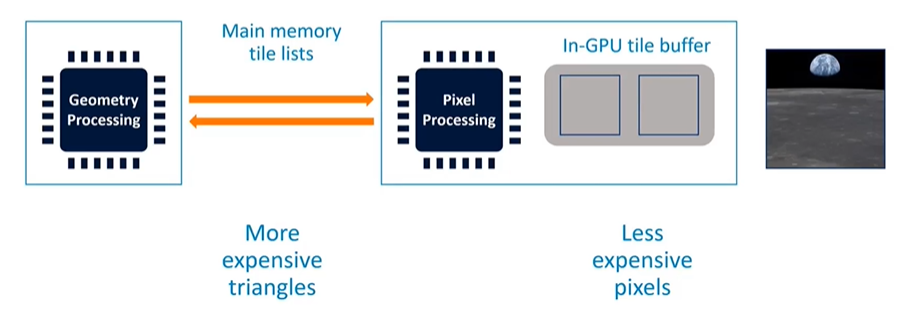
Tile-based rendering differs significantly from immediate mode rendering. In this method, the GPU must first complete all geometry processing to determine which triangles contribute to each tile. Given the complexity of modern graphics, this can involve processing up to half a million triangles, which is too much data to store on-chip. Consequently, this data is written back to main memory, combining vertex data with a tile list that tracks which triangles affect each tile.

On the pixel processing side, tiles are small enough that their working sets—color, depth, stencil, and multi-sample data—can be stored entirely within the GPU's RAM. This allows for efficient processing, as data remains within the GPU and only the final rendered tiles are written back to memory. For example, if depth testing is turned on but the data isn’t needed after rendering, it can be discarded without ever writing it back to main memory, leading to significant power savings.

Trade-Offs in Tile-Based Architecture

The tile-based approach involves two separate pipelines, with a main memory pass in between. This design trades off triangle efficiency for pixel efficiency. Triangles become more expensive to process because they are stored in main memory, but pixel processing is more efficient as the frame buffer stays within the GPU, closely coupled with the shader cores.

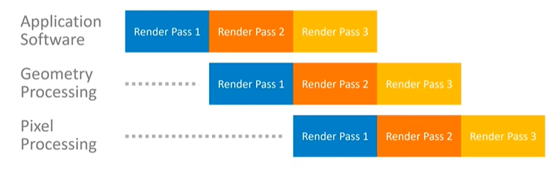
The pipelining behavior in tile-based architectures is also different. Render passes must be completed in full before pixel processing can begin, meaning the pipeline operates at a coarser level compared to immediate mode rendering. Although it is possible to overlap render passes, achieving this requires stricter adherence to application programming interface (API) rules.

Why Tile-Based Rendering for Mobile?

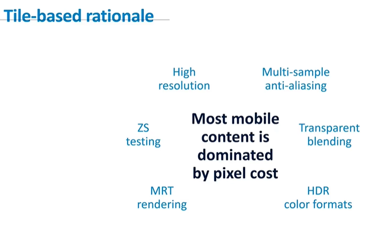
Tile-based rendering is particularly suited to mobile devices because mobile content is often pixel-intensive. With a significant amount of 2D content, layers, casual gaming, and lightweight 3D content, mobile applications are dominated by pixel costs rather than triangle complexity. By focusing on making pixel processing as energy-efficient as possible, tile-based architectures are well-suited for mobile environments where power consumption is a critical concern.

Advantages and Limitations of Tile-Based Rendering

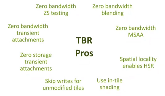
Tile-based rendering offers several advantages, especially concerning frame buffer operations. For instance, it allows for zero-bandwidth depth testing, blending, and multi-sampling if the data does not need to be stored in main memory. Techniques like hidden surface removal are more effective, and in-tile shading can be efficiently executed. These benefits stem from the close proximity of the small tile RAM to the shader core.

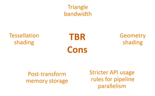
However, there are downsides. Triangles become more expensive to process as they need to be written to and read from main memory multiple times during the rendering process. Techniques like tessellation and geometry shading, which are well-suited to immediate mode architectures, are less efficient in a tile-based setup. These techniques require reading a simple model, expanding it with tessellation, and then writing the expanded data back to memory, making them costly in terms of memory bandwidth.

Implementation Spectrum and Variations

It’s important to note that GPU architectures exist on a spectrum between the archetypal immediate mode and tile-based renderers. While Mali GPUs represent a strict tile-based approach, other vendors may adopt hybrid methods that combine elements of both architectures. For example, some desktop GPUs are incorporating speculative tile-based techniques, and other mobile GPUs, like Adreno, may use larger tile sizes than Mali.

Conclusion

Understanding the strengths and weaknesses of tile-based rendering is crucial for developers, especially when creating content for mobile devices. The choice of GPU architecture has a significant impact on how applications are designed and optimized, particularly in terms of memory management and processing efficiency.

Upcoming: Shader Core Architecture

In the final part of today's discussion, we'll explore the hardware shader cores. This segment will cover how these cores are built and how their design differs from CPU cores, which will have implications for how we write shader programs.

Introduction to CPU and GPU Architecture

Most people who work in engineering or computer science are familiar with CPU architecture, having studied it during university or college. To understand GPU architecture, it's helpful to start with a CPU and then evolve that understanding into how a GPU works.

The Problem Domain of CPUs

A CPU is classified by the problem domain it aims to solve. Traditional CPUs are designed to handle relatively low-thread-count, long-running programs that execute control plane code. Even in parallel applications on a CPU, you typically only have 16 to 32 threads, not hundreds or thousands. The types of problems CPUs solve often don't parallelize well. Therefore, to make an application faster on a CPU, the focus is on making those few threads run quicker, often by increasing the CPU's clock rate.

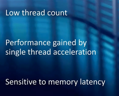
Sensitivity to Memory Latency

CPUs are highly sensitive to memory latency. If a CPU encounters a cache miss, it might take 200 cycles to access DRAM and retrieve the required data. During this time, the CPU has limited other work to do, making it very sensitive to cache misses and related delays.

CPU Pipeline and Instruction Processing

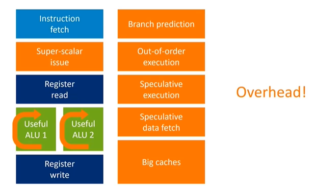
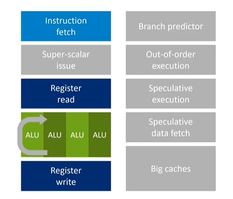
The essential components of a CPU include instruction fetch and decode, register read to fetch operands, a pipeline that performs useful work, and finally, writing results back to registers. CPUs often break down complex operations, like floating-point multiplications, into multi-stage pipelines to increase processing frequency. However, this adds latency to getting results.

To mitigate this latency, CPUs incorporate various hardware features:

1. Register Forwarding: This allows the CPU to loop back intermediate results within the pipeline, reducing result latency without having to go through the entire register read/write process.
2. Branch Prediction: To minimize delays caused by control flow changes, CPUs use branch predictors to guess the next instruction's address and start fetching and executing instructions before the current instruction has completed. If the prediction is wrong, the CPU must recover, adding extra hardware to hide pipeline latency.
3. Superscalar Execution: CPUs may execute multiple instructions in parallel, even though the instruction set architecture (ISA) is serial. This requires additional hardware to identify parallel execution opportunities among neighboring instructions.
4. Out-of-Order Execution: High-end CPUs often execute instructions out of order by examining a large window of instructions to find parallel execution opportunities, significantly increasing performance at the cost of added complexity.
5. Speculation: CPUs might prefetch data or fill idle slots based on guesses about future instructions.
6. Caches: Due to the high cost of these techniques, CPUs tend to have large caches (L1, L2) to store frequently accessed data, even though the actual programs may not be very large.

Energy Efficiency and Performance Trade-offs

All these features—the extra hardware for branch prediction, superscalar execution, out-of-order execution, and speculation—are necessary to keep the actual processing units (the green bits) busy. However, they consume significant energy. This is the primary difference between high-performance CPUs (like ARM's "big" CPUs) and energy-efficient ones (like ARM's "little" CPUs). The high-performance CPUs include more of this "orange stuff," which increases performance but decreases energy efficiency.

SIMD and Vector Processing

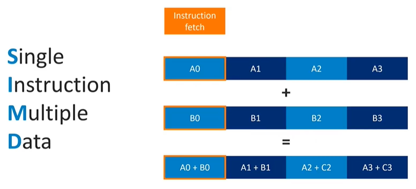
One particularly efficient feature in CPUs is SIMD (Single Instruction, Multiple Data), such as ARM's NEON technology. SIMD allows the CPU to execute a single instruction on multiple data points simultaneously. For example, a vector add operation (e.g., vec4 add) can process four parallel data operations with the same instruction fetch and control cost, effectively reducing the overhead. However, SIMD is only beneficial if the program includes instructions that can take advantage of this parallelism.

Transitioning to GPU Architecture

While SIMD and vector processing are useful in CPUs, GPUs take a different approach to parallelism. In the next section, we'll explore how GPUs are designed to handle massively parallel workloads, differentiating them from the CPU architecture described above.

Introduction to GPU Architecture

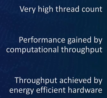
GPUs are fundamentally different from CPUs, primarily because the problem domain they address is vastly different. While CPUs are designed for low-thread-count, high-latency-sensitive tasks, GPUs handle extremely high-thread-count tasks, such as processing thousands or even millions of vertices and pixels, each running a unique vertex or fragment shader.

High Thread Count and Computational Throughput

In GPU workloads, the focus isn't on the latency of processing a single vertex or pixel but on the computational throughput of the entire problem space. This high degree of parallelism allows for very efficient hardware designs, where performance can be scaled simply by adding more cores. For example, mobile GPUs might have 20 shader cores, while desktop GPUs might have 128 shader cores, each capable of handling numerous threads simultaneously.

Parallelism and Efficient Core Design

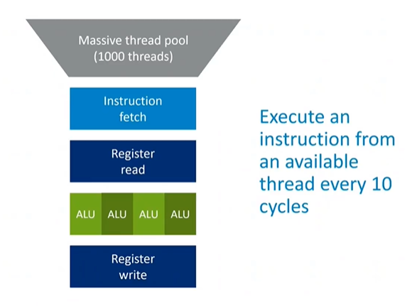
To illustrate GPU architecture, consider a CPU core with vector hardware at its center, taking 10 cycles to process from read to write. By exploiting the inherent parallelism in GPU tasks, a design could have 10 threads running concurrently in the core. Each cycle, a different thread is issued, so by the time the second instruction of the first thread is ready, the first instruction has already completed the pipeline. This design effectively hides pipeline length and removes the need for complex hardware such as superscalar issue, out-of-order execution, or speculation.

Simplified Hardware Requirements

In a GPU, since multiple threads are running simultaneously, there is no need for branch prediction or result forwarding. The next instruction in any thread can only run once the previous instruction has left the pipeline, so the results are already in registers. This means the costly hardware often required in high-end CPUs to handle these issues is not necessary in a GPU.

Handling Memory Latency

Memory latency, which can be over 100 cycles, is a significant challenge. However, with enough threads—say, 1,000 instead of just 10—a GPU can ensure that there is always at least one active thread ready to be issued every cycle. The other threads might be waiting for data from DRAM, but as long as there is a constant flow of threads being processed and data being requested and returned from memory, the GPU can effectively hide the cost of cache misses.

Vector Processing in GPUs

SIMD (Single Instruction, Multiple Data) operations are valuable in CPUs, but they only work when the application contains specific vector operations like vector add or multiply. In many cases, these SIMD instructions go unused because they don't fit all problems.

GPUs take a different approach to vector hardware. Instead of finding vector operations within a single thread, GPUs pack scalar operations from multiple threads together to create a vector operation. For instance, rather than executing a 4-wide vector add from one thread, a GPU might execute four scalar adds from four different threads simultaneously, using the same vector unit.

This method ensures that the vector hardware is always utilized, regardless of whether the original problem had explicit vector operations. This approach further enhances the efficiency and parallelism of GPU architectures.

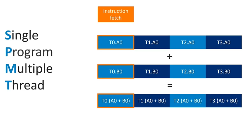
Vectorization in GPUs

In GPU architecture, multiple threads must originate from the same program and run the same program counter. Although there is no architectural guarantee that these threads form a vector, the hardware can still vectorize almost any operation. Even if a program contains only a scalar addition, by grouping four threads together, the GPU can fully utilize the vector hardware width. This approach allows the GPU to fetch and decode a single instruction while executing it across multiple threads in lockstep.

Thread Lockstep and Vectorization

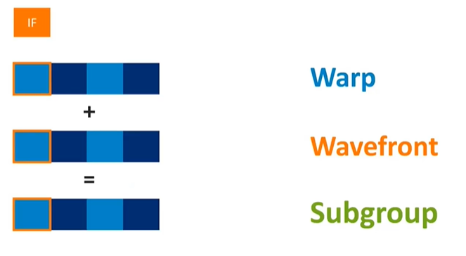
Running threads in lockstep—where all threads originate from the same draw call, vertex shader, or fragment shader program and share the same program counter during instruction issuance—is a common practice across contemporary GPUs. Different manufacturers use different terminology for this concept: NVIDIA calls them " ," AMD refers to them as "wavefronts," Vulkan specification names them "subgroups," and in Mali, they are generally termed "warps." Regardless of the terminology, the concept remains consistent: threads are grouped together in lockstep to leverage vector hardware, offering the benefits of vector processing while maintaining the flexibility of a scalar instruction stream.

Advantages of Wide Vector Units

By vectorizing operations across multiple threads, GPUs can make their vector units significantly wider. Given the abundance of threads in each draw call, GPUs can extend the width of vector units, thereby reducing the overhead associated with fetching and decoding instructions. For instance, if a GPU has a 4-wide vector unit, the orange overhead (control logic) is amortized over four threads. This concept can be extended to 16-wide or even wider units, further distributing the control overhead and enhancing efficiency. For example, the latest Mali GPUs feature 16-wide warps, allowing for a more efficient execution by averaging out the cost over a larger number of operations.

Challenges with Divergent Threads

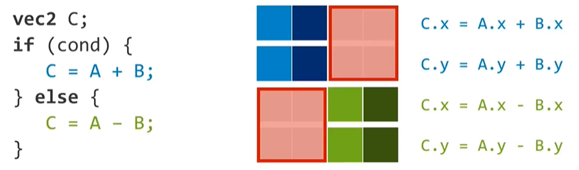
Running threads in lockstep also presents challenges, particularly when dealing with divergent control flow. If an "if-else" statement causes some threads to execute the "if" path and others to execute the "else" path, the GPU hardware must mask out the inactive lanes. In this case, the threads on the inactive path represent idle hardware, which can lead to inefficiencies. Therefore, minimizing divergence in control plane code is crucial in warp architectures to maintain efficiency and avoid accumulating unnecessary costs.

Fixed-Function Accelerators in Mobile GPUs

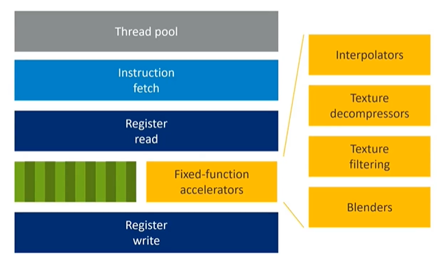
In mobile GPUs, fixed-function accelerators play a critical role. These accelerators handle specific tasks such as interpolation, texture decompression, texture filtering, and fixed-function blending. By exploiting the problem domain, GPUs can perform certain tasks with reduced precision (e.g., using fixed-point instead of floating-point calculations), saving energy and reducing transistor toggling. Although this requires additional silicon area, the overall energy efficiency is improved.

Conclusion

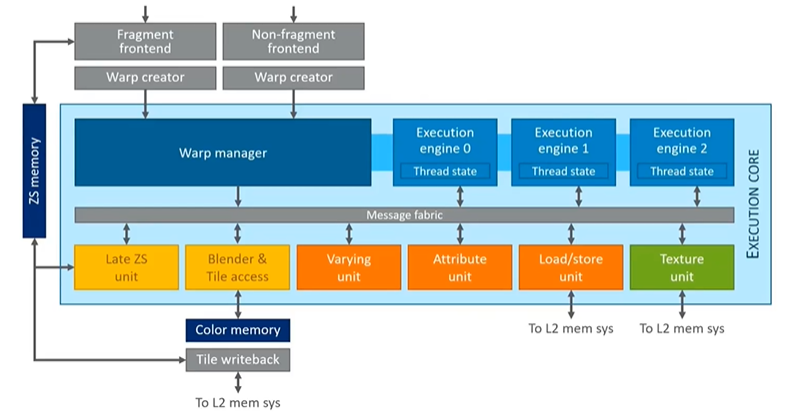
Bringing these elements together results in the design of a typical Mali shader core. This core includes various processing units, such as the arithmetic units highlighted in blue and numerous fixed-function hardware components along the bottom, dedicated to specific GPU tasks. Only the units in blue are responsible for running programs, while the fixed-function hardware accelerates other processes. These concepts and designs will be explored in greater detail tomorrow.